Computation of Frobenius matrix on Monsky-Washnitzer cohomology.¶

The most interesting functions to be exported here are matrix_of_frobenius() and adjusted_prec().

Currently this code is limited to the case $p \geq 5$ (no $GF(p^n)$ for $n > 1$ ), and only handles the elliptic curve case (not more general hyperelliptic curves).

REFERENCES:

Kedlaya, K., “Counting points on hyperelliptic curves using Monsky-Washnitzer cohomology”, J. Ramanujan Math. Soc. 16 (2001) no 4, 323-338
Edixhoven, B., “Point counting after Kedlaya”, EIDMA-Stieltjes graduate course, Lieden (lecture notes?).

AUTHORS:

David Harvey and Robert Bradshaw: initial code developed at the 2006 MSRI graduate workshop, working with Jennifer Balakrishnan and Liang Xiao
David Harvey (2006-08): cleaned up, rewrote some chunks, lots more documentation, added Newton iteration method, added more complete ‘trace trick’, integrated better into Sage.
David Harvey (2007-02): added algorithm with sqrt(p) complexity (removed in May 2007 due to better C++ implementation)
Robert Bradshaw (2007-03): keep track of exact form in reduction algorithms
Robert Bradshaw (2007-04): generalization to hyperelliptic curves

class sage.schemes.elliptic_curves.monsky_washnitzer.MonskyWashnitzerDifferential(parent, val=0, offset=0)¶

Bases: sage.structure.element.ModuleElement

Represents an element of the form F dx/2y

coeff()¶: This is a one-dimensional module over the base ring, generated by dx/2y. Return $A$ where $A dx/2y = self$ .

coeffs(R=None)¶

coleman_integral(P, Q)¶

extract_pow_y(k)¶: Really the power of y in A where self = A dx/2y.

integrate(P, Q)¶

max_pow_y()¶: Really the maximum power of y in A where self = A dx/2y.

min_pow_y()¶: Really the minimum power of y in A where self = A dx/2y.

reduce()¶: Use homology relations to find $a$ and $f$ such that $self = a + df$ where $a$ is given in terms of the $x^i dx/2y$ .

reduce_fast(even_degree_only=False)¶

Use homology relations to find $a$ and $f$ such that $self = a + df$ where $a$ is given in terms of the $x^i dx/2y$ .

EXAMPLES:

sage: R.<x> = QQ['x']
sage: E = HyperellipticCurve(x^3-4*x+4)
sage: x, y = E.monsky_washnitzer_gens()
sage: x.diff().reduce_fast()
(x, (0, 0))
sage: y.diff().reduce_fast()
(y*1, (0, 0))
sage: (y^-1).diff().reduce_fast()
((y^-1)*1, (0, 0))
sage: (y^-11).diff().reduce_fast()
((y^-11)*1, (0, 0))
sage: (x*y^2).diff().reduce_fast()
(y^2*x, (0, 0))

reduce_neg_y()¶: Use homology relations to eliminate negative powers of y.

reduce_neg_y_fast(even_degree_only=False)¶

Use homology relations to eliminate negative powers of y.

EXAMPLES:

sage: R.<x> = QQ['x']
sage: E = HyperellipticCurve(x^5-3*x+1)
sage: x, y = E.monsky_washnitzer_gens()
sage: (y^-1).diff().reduce_neg_y_fast()
((y^-1)*1, 0 dx/2y)
sage: (y^-5*x^2+y^-1*x).diff().reduce_neg_y_fast()
((y^-1)*x + (y^-5)*x^2, 0 dx/2y)            

It leaves non-negative powers of y alone:

sage: y.diff()
((-3)*1 + 5*x^4) dx/2y
sage: y.diff().reduce_neg_y_fast()
(0, ((-3)*1 + 5*x^4) dx/2y)

reduce_neg_y_faster(even_degree_only=False)¶: Use homology relations to eliminate negative powers of y.

reduce_pos_y()¶: Use homology relations to eliminate positive powers of y.

reduce_pos_y_fast(even_degree_only=False)¶

Use homology relations to eliminate positive powers of y.

EXAMPLES:

sage: R.<x> = QQ['x']
sage: E = HyperellipticCurve(x^3-4*x+4)
sage: x, y = E.monsky_washnitzer_gens()
sage: y.diff().reduce_pos_y_fast()
(y*1, 0 dx/2y)
sage: (y^2).diff().reduce_pos_y_fast()
(y^2*1, 0 dx/2y)
sage: (y^2*x).diff().reduce_pos_y_fast()
(y^2*x, 0 dx/2y)
sage: (y^92*x).diff().reduce_pos_y_fast()
(y^92*x, 0 dx/2y)
sage: w = (y^3 + x).diff()
sage: w += w.parent()(x)
sage: w.reduce_pos_y_fast()
(y^3*1 + x, x dx/2y)

sage.schemes.elliptic_curves.monsky_washnitzer.MonskyWashnitzerDifferentialRing(base_ring)¶

class sage.schemes.elliptic_curves.monsky_washnitzer.MonskyWashnitzerDifferentialRing_class(base_ring)¶

Bases: sage.modules.module.Module

Q()¶

base_extend(R)¶

change_ring(R)¶

degree()¶

frob_Q(p)¶

frob_basis_elements(prec, p)¶

frob_invariant_differential(prec, p)¶: $F_p(dx/y) = px^{p-1} y(F_py)^{-1} dx/y = px^{p-1} y^{1-p} (1+pEy^{-2p})^{-1/2} dx/y = px^{p-1} y^{1-p} (F_pQ y^{-p})^{-1/2} dx/y$

Use Newton’s method to calculate the square root.

helper_matrix()¶: We use this to solve for the linear combination of $x^i y^j$ needed to clear all terms with $y^{j-1}$ .

invariant_differential()¶

x_to_p(p)¶

class sage.schemes.elliptic_curves.monsky_washnitzer.SpecialCubicQuotientRing(Q, laurent_series=False)¶

Bases: sage.rings.ring.CommutativeAlgebra

Specialised class for representing the quotient ring $R[x,T]/(T - x^3 - ax - b)$ , where $R$ is an arbitrary commutative base ring (in which 2 and 3 are invertible), $a$ and $b$ are elements of that ring.

Polynomials are represented internally in the form $p_0 + p_1 x + p_2 x^2$ where the $p_i$ are polynomials in $T$ . Multiplication of polynomials always reduces high powers of $x$ (i.e. beyond $x^2$ ) to powers of $T$ .

Hopefully this ring is faster than a general quotient ring because it uses the special structure of this ring to speed multiplication (which is the dominant operation in the frobenius matrix calculation). I haven’t actually tested this theory though...

TODO: - Eventually we will want to run this in characteristic 3, so we need to: (a) Allow Q(x) to contain an $x^2$ term, and (b) Remove the requirement that 3 be invertible. Currently this is used in the Toom-Cook algorithm to speed multiplication.

EXAMPLES:

sage: B.<t> = PolynomialRing(Integers(125))
sage: R = monsky_washnitzer.SpecialCubicQuotientRing(t^3 - t + B(1/4))
sage: R
SpecialCubicQuotientRing over Ring of integers modulo 125 with polynomial T = x^3 + 124*x + 94

Get generators:

sage: x, T = R.gens()
sage: x
(0) + (1)*x + (0)*x^2
sage: T
(T) + (0)*x + (0)*x^2

Coercions:

sage: R(7)
(7) + (0)*x + (0)*x^2

Create elements directly from polynomials:

sage: A, z = R.poly_ring().objgen()
sage: A
Univariate Polynomial Ring in T over Ring of integers modulo 125
sage: R.create_element(z^2, z+1, 3)
(T^2) + (T + 1)*x + (3)*x^2

Some arithmetic:

sage: x^3
(T + 31) + (1)*x + (0)*x^2
sage: 3 * x**15 * T**2 + x - T
(3*T^7 + 90*T^6 + 110*T^5 + 20*T^4 + 58*T^3 + 26*T^2 + 124*T) + (15*T^6 + 110*T^5 + 35*T^4 + 63*T^2 + 1)*x + (30*T^5 + 40*T^4 + 8*T^3 + 38*T^2)*x^2

Retrieve coefficients (output is zero-padded):

sage: x^10
(3*T^2 + 61*T + 8) + (T^3 + 93*T^2 + 12*T + 40)*x + (3*T^2 + 61*T + 9)*x^2
sage: (x^10).coeffs()
[[8, 61, 3, 0], [40, 12, 93, 1], [9, 61, 3, 0]]

TODO: write an example checking multiplication of these polynomials against Sage’s ordinary quotient ring arithmetic. I can’t seem to get the quotient ring stuff happening right now...

create_element(p0, p1, p2, check=True)¶

Creates the element $p_0 + p_1*x + p_2*x^2$ , where pi’s are polynomials in T.

INPUT:

p0, p1, p2 - coefficients; must be coercible into poly_ring()
check - bool (default True): whether to carry out coercion

EXAMPLES:

sage: B.<t> = PolynomialRing(Integers(125))
sage: R = monsky_washnitzer.SpecialCubicQuotientRing(t^3 - t + B(1/4))
sage: A, z = R.poly_ring().objgen()
sage: R.create_element(z^2, z+1, 3)
(T^2) + (T + 1)*x + (3)*x^2

gens()¶

Return a list [x, T] where x and T are the generators of the ring (as element of this ring).

Note

I have no idea if this is compatible with the usual Sage ‘gens’ interface.

EXAMPLES:

sage: B.<t> = PolynomialRing(Integers(125))
sage: R = monsky_washnitzer.SpecialCubicQuotientRing(t^3 - t + B(1/4))
sage: x, T = R.gens()
sage: x
(0) + (1)*x + (0)*x^2
sage: T
(T) + (0)*x + (0)*x^2

poly_ring()¶

Return the underlying polynomial ring in T.

EXAMPLES:

sage: B.<t> = PolynomialRing(Integers(125))
sage: R = monsky_washnitzer.SpecialCubicQuotientRing(t^3 - t + B(1/4))
sage: R.poly_ring()
Univariate Polynomial Ring in T over Ring of integers modulo 125

class sage.schemes.elliptic_curves.monsky_washnitzer.SpecialCubicQuotientRingElement(parent, p0, p1, p2, check=True)¶

Bases: sage.structure.element.CommutativeAlgebraElement

An element of a SpecialCubicQuotientRing.

coeffs()¶

Returns list of three lists of coefficients, corresponding to the $x^0$ , $x^1$ , $x^2$ coefficients. The lists are zero padded to the same length. The list entries belong to the base ring.

EXAMPLES:

sage: B.<t> = PolynomialRing(Integers(125))
sage: R = monsky_washnitzer.SpecialCubicQuotientRing(t^3 - t + B(1/4))
sage: p = R.create_element(t, t^2 - 2, 3)
sage: p.coeffs()
[[0, 1, 0], [123, 0, 1], [3, 0, 0]]

scalar_multiply(scalar)¶

Multiplies this element by a scalar, i.e. just multiply each coefficient of $x^j$ by the scalar.

INPUT:

scalar - either an element of base_ring, or an element of poly_ring.

EXAMPLES:

sage: B.<t> = PolynomialRing(Integers(125))
sage: R = monsky_washnitzer.SpecialCubicQuotientRing(t^3 - t + B(1/4))
sage: x, T = R.gens()
sage: f = R.create_element(2, t, t^2 - 3)
sage: f
(2) + (T)*x + (T^2 + 122)*x^2
sage: f.scalar_multiply(2)
(4) + (2*T)*x + (2*T^2 + 119)*x^2
sage: f.scalar_multiply(t)
(2*T) + (T^2)*x + (T^3 + 122*T)*x^2

shift(n)¶

Returns this element multiplied by $T^n$ .

EXAMPLES:

sage: B.<t> = PolynomialRing(Integers(125))
sage: R = monsky_washnitzer.SpecialCubicQuotientRing(t^3 - t + B(1/4))
sage: f = R.create_element(2, t, t^2 - 3)
sage: f
(2) + (T)*x + (T^2 + 122)*x^2
sage: f.shift(1)
(2*T) + (T^2)*x + (T^3 + 122*T)*x^2
sage: f.shift(2)
(2*T^2) + (T^3)*x + (T^4 + 122*T^2)*x^2

square()¶

EXAMPLES:

sage: B.<t> = PolynomialRing(Integers(125))
sage: R = monsky_washnitzer.SpecialCubicQuotientRing(t^3 - t + B(1/4))
sage: x, T = R.gens()

sage: f = R.create_element(1 + 2*t + 3*t^2, 4 + 7*t + 9*t^2, 3 + 5*t + 11*t^2)
sage: f.square()
(73*T^5 + 16*T^4 + 38*T^3 + 39*T^2 + 70*T + 120) + (121*T^5 + 113*T^4 + 73*T^3 + 8*T^2 + 51*T + 61)*x + (18*T^4 + 60*T^3 + 22*T^2 + 108*T + 31)*x^2

class sage.schemes.elliptic_curves.monsky_washnitzer.SpecialHyperellipticQuotientElement(parent, val=0, offset=0, check=True)¶

Bases: sage.structure.element.CommutativeAlgebraElement

change_ring(R)¶

coeffs(R=None)¶

diff()¶

extract_pow_y(k)¶

max_pow_y()¶

min_pow_y()¶

truncate_neg(n)¶

sage.schemes.elliptic_curves.monsky_washnitzer.SpecialHyperellipticQuotientRing(*args)¶

class sage.schemes.elliptic_curves.monsky_washnitzer.SpecialHyperellipticQuotientRing_class(Q, R=None, invert_y=True)¶

Bases: sage.rings.ring.CommutativeAlgebra

Q()¶

base_extend(R)¶

change_ring(R)¶

curve()¶

degree()¶

gens()¶

is_field(proof=True)¶

monomial(i, j, b=None)¶: Returns $b y^j x^i$ , computed quickly.

monomial_diff_coeffs(i, j)¶

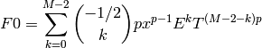
The key here is that the formula for $d(x^iy^j)$ is messy in terms of i, but varies nicely with j.

$d(x^iy^j) = y^{j-1} (2ix^{i-1}y^2 + j (A_i(x) + B_i(x)y^2)) \frac{dx}{2y}$

Where $A,B$ have degree at most $n-1$ for each $i$ . Pre-compute $A_i, B_i$ for each $i$ the “hard” way, and the rest are easy.

monomial_diff_coeffs_matrices()¶

monsky_washnitzer()¶

prime()¶

x()¶

y()¶

sage.schemes.elliptic_curves.monsky_washnitzer.adjusted_prec(p, prec)¶

Computes how much precision is required in matrix_of_frobenius to get an answer correct to prec $p$ -adic digits.

The issue is that the algorithm used in matrix_of_frobenius sometimes performs divisions by $p$ , so precision is lost during the algorithm.

The estimate returned by this function is based on Kedlaya’s result (Lemmas 2 and 3 of “Counting Points on Hyperelliptic Curves...”), which implies that if we start with $M$ $p$ -adic digits, the total precision loss is at most $1 + \lfloor \log_p(2M-3) \rfloor$ $p$ -adic digits. (This estimate is somewhat less than the amount you would expect by naively counting the number of divisions by $p$ .)

INPUT:

p - a prime = 5
prec - integer, desired output precision, = 1

OUTPUT: adjusted precision (usually slightly more than prec)

sage.schemes.elliptic_curves.monsky_washnitzer.frobenius_expansion_by_newton(Q, p, M)¶

Computes the action of Frobenius on $dx/y$ and on $x dx/y$ , using Newton’s method (as suggested in Kedlaya’s paper).

(This function does not yet use the cohomology relations - that happens afterwards in the “reduction” step.)

More specifically, it finds $F_0$ and $F_1$ in the quotient ring $R[x, T]/(T - Q(x))$ , such that

$F( dx/y) = T^{-r} F0 dx/y, \text{\ and\ } F(x dx/y) = T^{-r} F1 dx/y$

where

$r = ( (2M-3)p - 1 )/2.$

(Here $T$ is $y^2 = z^{-2}$ , and $R$ is the coefficient ring of $Q$ .)

$F_0$ and $F_1$ are computed in the SpecialCubicQuotientRing associated to $Q$ , so all powers of $x^j$ for $j \geq 3$ are reduced to powers of $T$ .

INPUT:

Q - cubic polynomial of the form $Q(x) = x^3 + ax + b$ , whose coefficient ring is a $Z/(p^M)Z$ -algebra
p - residue characteristic of the p-adic field
M - p-adic precision of the coefficient ring (this will be used to determine the number of Newton iterations)

OUTPUT:

F0, F1 - elements of SpecialCubicQuotientRing(Q), as described above
r - non-negative integer, as described above

sage.schemes.elliptic_curves.monsky_washnitzer.frobenius_expansion_by_series(Q, p, M)¶

Computes the action of Frobenius on dx/y and on x dx/y, using a series expansion.

(This function computes the same thing as frobenius_expansion_by_newton(), using a different method. Theoretically the Newton method should be asymptotically faster, when the precision gets large. However, in practice, this functions seems to be marginally faster for moderate precision, so I’m keeping it here until I figure out exactly why it’s faster.)

(This function does not yet use the cohomology relations - that happens afterwards in the “reduction” step.)

More specifically, it finds F0 and F1 in the quotient ring $R[x, T]/(T - Q(x))$ , such that $F( dx/y) = T^{-r} F0 dx/y$ , and $F(x dx/y) = T^{-r} F1 dx/y$ where $r = ( (2M-3)p - 1 )/2$ . (Here T is $y^2 = z^{-2}$ , and R is the coefficient ring of Q.)

$F_0$ and $F_1$ are computed in the SpecialCubicQuotientRing associated to $Q$ , so all powers of $x^j$ for $j \geq 3$ are reduced to powers of $T$ .

It uses the sum

$F0 = \sum_{k=0}^{M-2} {-1/2 \choose k} p x^{p-1} E^k T^{(M-2-k)p}$

and

$F1 = x^p F0, where `E = Q(x^p) - Q(x)^p`.$

INPUT:

Q - cubic polynomial of the form $Q(x) = x^3 + ax + b$ , whose coefficient ring is a $\ZZ/(p^M)\ZZ$ -algebra
p - residue characteristic of the p-adic field
M - p-adic precision of the coefficient ring (this will be used to determine the number of terms in the series)

OUTPUT:

F0, F1 - elements of SpecialCubicQuotientRing(Q), as described above
r - non-negative integer, as described above

sage.schemes.elliptic_curves.monsky_washnitzer.helper_matrix(Q)¶

Computes the (constant) matrix used to calculate the linear combinations of the $d(x^i y^j)$ needed to eliminate the negative powers of $y$ in the cohomology (i.e. in reduce_negative()).

INPUT:

Q - cubic polynomial

sage.schemes.elliptic_curves.monsky_washnitzer.lift(x)¶

Tries to call x.lift(), presumably from the p-adics to ZZ.

If this fails, it assumes the input is a power series, and tries to lift it to a power series over QQ.

This function is just a very kludgy solution to the problem of trying to make the reduction code (below) work over both Zp and Zp[[t]].

sage.schemes.elliptic_curves.monsky_washnitzer.matrix_of_frobenius(Q, p, M, trace=None, compute_exact_forms=False)¶

Computes the matrix of Frobenius on Monsky-Washnitzer cohomology, with respect to the basis $(dx/y, x dx/y)$ .

INPUT:

Q - cubic polynomial $Q(x) = x^3 + ax + b$ defining an elliptic curve E by $y^2 = Q(x)$ . The coefficient ring of Q should be a $\ZZ/(p^M)\ZZ$ -algebra in which the matrix of frobenius will be constructed.
p - prime = 5 for which E has good reduction
M - integer = 2; $p$ -adic precision of the coefficient ring
trace - (optional) the trace of the matrix, if known in advance. This is easy to compute because it’s just the $a_p$ of the curve. If the trace is supplied, matrix_of_frobenius will use it to speed the computation (i.e. we know the determinant is $p$ , so we have two conditions, so really only column of the matrix needs to be computed. It’s actually a little more complicated than that, but that’s the basic idea.) If trace=None, then both columns will be computed independently, and you can get a strong indication of correctness by verifying the trace afterwards.

Warning

THE RESULT WILL NOT NECESSARILY BE CORRECT TO M p-ADIC DIGITS. If you want prec digits of precision, you need to use the function adjusted_prec(), and then you need to reduce the answer mod $p^{\mathrm{prec}}$ at the end.

OUTPUT: 2x2 matrix of frobenius on Monsky-Washnitzer cohomology, with entries in the coefficient ring of Q.

EXAMPLES: A simple example:

sage: p = 5
sage: prec = 3
sage: M = monsky_washnitzer.adjusted_prec(p, prec)
sage: M
5
sage: R.<x> = PolynomialRing(Integers(p**M))
sage: A = monsky_washnitzer.matrix_of_frobenius(x^3 - x + R(1/4), p, M)
sage: A
[3090  187]
[2945  408]

But the result is only accurate to prec digits:

sage: B = A.change_ring(Integers(p**prec))
sage: B
[90 62]
[70 33]

Check trace (123 = -2 mod 125) and determinant:

sage: B.det()
5
sage: B.trace()
123
sage: EllipticCurve([-1, 1/4]).ap(5)
-2

Try using the trace to speed up the calculation:

sage: A = monsky_washnitzer.matrix_of_frobenius(x^3 - x + R(1/4),
...                                             p, M, -2)
sage: A
[2715  187]
[1445  408]

Hmmm... it looks different, but that’s because the trace of our first answer was only -2 modulo $5^3$ , not -2 modulo $5^5$ . So the right answer is:

sage: A.change_ring(Integers(p**prec))
     [90 62]
     [70 33]

Check it works with only one digit of precision:

sage: p = 5
sage: prec = 1
sage: M = monsky_washnitzer.adjusted_prec(p, prec)
sage: R.<x> = PolynomialRing(Integers(p**M))
sage: A = monsky_washnitzer.matrix_of_frobenius(x^3 - x + R(1/4), p, M)
sage: A.change_ring(Integers(p))
[0 2]
[0 3]

Here’s an example that’s particularly badly conditioned for using the trace trick:

sage: p = 11
sage: prec = 3
sage: M = monsky_washnitzer.adjusted_prec(p, prec)
sage: R.<x> = PolynomialRing(Integers(p**M))
sage: A = monsky_washnitzer.matrix_of_frobenius(x^3 + 7*x + 8, p, M)
sage: A.change_ring(Integers(p**prec))
[1144  176]
[ 847  185]

The problem here is that the top-right entry is divisible by 11, and the bottom-left entry is divisible by $11^2$ . So when you apply the trace trick, neither $F(dx/y)$ nor $F(x dx/y)$ is enough to compute the whole matrix to the desired precision, even if you try increasing the target precision by one. Nevertheless, matrix_of_frobenius knows how to get the right answer by evaluating $F((x+1) dx/y)$ instead:

sage: A = monsky_washnitzer.matrix_of_frobenius(x^3 + 7*x + 8, p, M, -2)
sage: A.change_ring(Integers(p**prec))
[1144  176]
[ 847  185]

The running time is about O(p*prec**2) (times some logarithmic factors), so it’s feasible to run on fairly large primes, or precision (or both?!?!):

sage: p = 10007
sage: prec = 2
sage: M = monsky_washnitzer.adjusted_prec(p, prec)
sage: R.<x> = PolynomialRing(Integers(p**M))
sage: A = monsky_washnitzer.matrix_of_frobenius(            # long time
...                             x^3 - x + R(1/4), p, M)     # long time
sage: B = A.change_ring(Integers(p**prec)); B               # long time
[74311982 57996908]
[95877067 25828133]
sage: B.det()                                               # long time
10007
sage: B.trace()                                             # long time
66
sage: EllipticCurve([-1, 1/4]).ap(10007)                    # long time
66

sage: p = 5
sage: prec = 300
sage: M = monsky_washnitzer.adjusted_prec(p, prec)
sage: R.<x> = PolynomialRing(Integers(p**M))
sage: A = monsky_washnitzer.matrix_of_frobenius(            # long time
...                             x^3 - x + R(1/4), p, M)     # long time
sage: B = A.change_ring(Integers(p**prec))                  # long time
sage: B.det()                                               # long time
5
sage: -B.trace()                                            # long time
2
sage: EllipticCurve([-1, 1/4]).ap(5)                        # long time
-2

Let’s check consistency of the results for a range of precisions:

sage: p = 5
sage: max_prec = 60
sage: M = monsky_washnitzer.adjusted_prec(p, max_prec)
sage: R.<x> = PolynomialRing(Integers(p**M))
sage: A = monsky_washnitzer.matrix_of_frobenius(x^3 - x + R(1/4), p, M)         # long time
sage: A = A.change_ring(Integers(p**max_prec))              # long time
sage: result = []                                           # long time
sage: for prec in range(1, max_prec):                       # long time
...       M = monsky_washnitzer.adjusted_prec(p, prec)      # long time
...       R.<x> = PolynomialRing(Integers(p^M),'x')         # long time
...       B = monsky_washnitzer.matrix_of_frobenius(        # long time
...                         x^3 - x + R(1/4), p, M)         # long time
...       B = B.change_ring(Integers(p**prec))              # long time
...       result.append(B == A.change_ring(                 # long time
...                                Integers(p**prec)))      # long time
sage: result == [True] * (max_prec - 1)                     # long time
True

The remaining examples discuss what happens when you take the coefficient ring to be a power series ring; i.e. in effect you’re looking at a family of curves.

The code does in fact work...

sage: p = 11
sage: prec = 3
sage: M = monsky_washnitzer.adjusted_prec(p, prec)
sage: S.<t> = PowerSeriesRing(Integers(p**M), default_prec=4)
sage: a = 7 + t + 3*t^2
sage: b = 8 - 6*t + 17*t^2
sage: R.<x> = PolynomialRing(S)
sage: Q = x**3 + a*x + b
sage: A = monsky_washnitzer.matrix_of_frobenius(Q, p, M)    # long time
sage: B = A.change_ring(PowerSeriesRing(Integers(p**prec), 't', default_prec=4))        # long time
sage: B                                                     # long time
[1144 + 264*t + 841*t^2 + 1025*t^3 + O(t^4)  176 + 1052*t + 216*t^2 + 523*t^3 + O(t^4)]
[   847 + 668*t + 81*t^2 + 424*t^3 + O(t^4)   185 + 341*t + 171*t^2 + 642*t^3 + O(t^4)]

The trace trick should work for power series rings too, even in the badly- conditioned case. Unfortunately I don’t know how to compute the trace in advance, so I’m not sure exactly how this would help. Also, I suspect the running time will be dominated by the expansion, so the trace trick won’t really speed things up anyway. Another problem is that the determinant is not always p:

sage: B.det()                                               # long time
11 + 484*t^2 + 451*t^3 + O(t^4)

However, it appears that the determinant always has the property that if you substitute t - 11t, you do get the constant series p (mod p**prec). Similarly for the trace. And since the parameter only really makes sense when it’s divisible by p anyway, perhaps this isn’t a problem after all.

sage.schemes.elliptic_curves.monsky_washnitzer.matrix_of_frobenius_hyperelliptic(Q, p=None, prec=None, M=None)¶

sage.schemes.elliptic_curves.monsky_washnitzer.reduce_all(Q, p, coeffs, offset, compute_exact_form=False)¶

Applies cohomology relations to reduce all terms to a linear combination of $dx/y$ and $x dx/y$ .

INPUT:

Q - cubic polynomial
coeffs - list of length 3 lists. The $i^{th}$ list [a, b, c] represents $y^{2(i - offset)} (a + bx + cx^2) dx/y$ .
offset - nonnegative integer

OUTPUT:

A, B - pair such that the input differential is cohomologous to (A + Bx) dx/y.

Note

The algorithm operates in-place, so the data in coeffs is destroyed.

EXAMPLE:

sage: R.<x> = Integers(5^3)['x']
sage: Q = x^3 - x + R(1/4)
sage: coeffs = [[1, 2, 3], [4, 5, 6], [7, 8, 9]]
sage: coeffs = [[R.base_ring()(a) for a in row] for row in coeffs]
sage: monsky_washnitzer.reduce_all(Q, 5, coeffs, 1)
 (21, 106)

sage.schemes.elliptic_curves.monsky_washnitzer.reduce_negative(Q, p, coeffs, offset, exact_form=None)¶

Applies cohomology relations to incorporate negative powers of $y$ into the $y^0$ term.

INPUT:

p - prime
Q - cubic polynomial
coeffs - list of length 3 lists. The $i^{th}$ list [a, b, c] represents $y^{2(i - offset)} (a + bx + cx^2) dx/y$ .
offset - nonnegative integer

OUTPUT: The reduction is performed in-place. The output is placed in coeffs[offset]. Note that coeffs[i] will be meaningless for i offset after this function is finished.

EXAMPLE:

sage: R.<x> = Integers(5^3)['x']
sage: Q = x^3 - x + R(1/4)
sage: coeffs = [[10, 15, 20], [1, 2, 3], [4, 5, 6], [7, 8, 9]]
sage: coeffs = [[R.base_ring()(a) for a in row] for row in coeffs]
sage: monsky_washnitzer.reduce_negative(Q, 5, coeffs, 3)
sage: coeffs[3]
 [28, 52, 9]

sage: R.<x> = Integers(7^3)['x']
sage: Q = x^3 - x + R(1/4)
sage: coeffs = [[7, 14, 21], [1, 2, 3], [4, 5, 6], [7, 8, 9]]
sage: coeffs = [[R.base_ring()(a) for a in row] for row in coeffs]
sage: monsky_washnitzer.reduce_negative(Q, 7, coeffs, 3)
sage: coeffs[3]
 [245, 332, 9]

sage.schemes.elliptic_curves.monsky_washnitzer.reduce_positive(Q, p, coeffs, offset, exact_form=None)¶

Applies cohomology relations to incorporate positive powers of $y$ into the $y^0$ term.

INPUT:

Q - cubic polynomial
coeffs - list of length 3 lists. The $i^{th}$ list [a, b, c] represents $y^{2(i - offset)} (a + bx + cx^2) dx/y$ .
offset - nonnegative integer

OUTPUT: The reduction is performed in-place. The output is placed in coeffs[offset]. Note that coeffs[i] will be meaningless for i offset after this function is finished.

EXAMPLE:

sage: R.<x> = Integers(5^3)['x']
sage: Q = x^3 - x + R(1/4)

sage: coeffs = [[1, 2, 3], [10, 15, 20]]
sage: coeffs = [[R.base_ring()(a) for a in row] for row in coeffs]
sage: monsky_washnitzer.reduce_positive(Q, 5, coeffs, 0)
sage: coeffs[0]
 [16, 102, 88]

sage: coeffs = [[9, 8, 7], [10, 15, 20]]
sage: coeffs = [[R.base_ring()(a) for a in row] for row in coeffs]
sage: monsky_washnitzer.reduce_positive(Q, 5, coeffs, 0)
sage: coeffs[0]
 [24, 108, 92]

sage.schemes.elliptic_curves.monsky_washnitzer.reduce_zero(Q, coeffs, offset, exact_form=None)¶

Applies cohomology relation to incorporate $x^2 y^0$ term into $x^0 y^0$ and $x^1 y^0$ terms.

INPUT:

Q - cubic polynomial
coeffs - list of length 3 lists. The $i^{th}$ list [a, b, c] represents $y^{2(i - offset)} (a + bx + cx^2) dx/y$ .
offset - nonnegative integer

OUTPUT: The reduction is performed in-place. The output is placed in coeffs[offset]. This method completely ignores coeffs[i] for i != offset.

EXAMPLE:

sage: R.<x> = Integers(5^3)['x']
sage: Q = x^3 - x + R(1/4)
sage: coeffs = [[1, 2, 3], [4, 5, 6], [7, 8, 9]]
sage: coeffs = [[R.base_ring()(a) for a in row] for row in coeffs]
sage: monsky_washnitzer.reduce_zero(Q, coeffs, 1)
sage: coeffs[1]
 [6, 5, 0]

sage.schemes.elliptic_curves.monsky_washnitzer.transpose_list(input)¶

INPUT:

input - a list of lists, each list of the same length

OUTPUT:

output - a list of lists such that output[i][j] = input[j][i]

EXAMPLES:

sage: from sage.schemes.elliptic_curves.monsky_washnitzer import transpose_list
sage: L = [[1, 2], [3, 4], [5, 6]]
sage: transpose_list(L)
[[1, 3, 5], [2, 4, 6]]

Computation of Frobenius matrix on Monsky-Washnitzer cohomology.¶

Previous topic

Next topic

This Page

Navigation

Computation of Frobenius matrix on Monsky-Washnitzer cohomology.¶

Previous topic

Next topic

This Page

Quick search

Navigation