Double Precision Complex Numbers¶

Sage supports arithmetic using double-precision complex numbers. A double-precision complex number is a complex number x + I*y with x, y 64-bit (8 byte) floating point numbers (double precision).

The field ComplexDoubleField implements the field of all double-precision complex numbers. You can refer to this field by the shorthand CDF. Elements of this field are of type ComplexDoubleElement. If x and y are coercible to doubles, you can create a complex double element using ComplexDoubleElement(x,y). You can coerce more general objects z to complex doubles by typing either ComplexDoubleField(x) or CDF(x).

EXAMPLES:

sage: ComplexDoubleField()
Complex Double Field
sage: CDF
Complex Double Field
sage: type(CDF.0)
<type 'sage.rings.complex_double.ComplexDoubleElement'>
sage: ComplexDoubleElement(sqrt(2),3)
1.41421356237 + 3.0*I
sage: parent(CDF(-2))
Complex Double Field

sage: CC == CDF
False
sage: CDF is ComplexDoubleField()     # CDF is the shorthand
True
sage: CDF == ComplexDoubleField()
True

The underlying arithmetic of complex numbers is implemented using functions and macros in GSL (the GNU Scientific Library), and should be very fast. Also, all standard complex trig functions, log, exponents, etc., are implemented using GSL, and are also robust and fast. Several other special functions, e.g. eta, gamma, incomplete gamma, etc., are implemented using the PARI C library.

AUTHORS:

William Stein (2006-09): first version

class sage.rings.complex_double.ComplexDoubleElement¶

Bases: sage.structure.element.FieldElement

An approximation to a complex number using double precision floating point numbers. Answers derived from calculations with such approximations may differ from what they would be if those calculations were performed with true complex numbers. This is due to the rounding errors inherent to finite precision calculations.

abs()¶

This function returns the magnitude of the complex number $z$ , $|z|$ .

EXAMPLES:

sage: CDF(2,3).abs()   # slightly random-ish arch dependent output
3.6055512754639891

abs2()¶

This function returns the squared magnitude of the complex number $z$ , $|z|^2$ .

EXAMPLES:

sage: CDF(2,3).abs2()
13.0

agm(right, algorithm='optimal')¶

Return the Arithmetic-Geometric Mean (AGM) of self and right.

INPUT:

right (complex) – another complex number
algorithm (string, default “optimal”) – the algorithm to use

(see below).

OUTPUT:

(complex) A value of the AGM of self and right. Note that this is a multi-valued function, and the algorithm used affects the value returned, as follows:

“pari”: Call the agm function from the pari library.
“optimal”: Use the AGM sequence such that at each stage

$(a,b)$ is replaced by $(a_1,b_1)=((a+b)/2,\pm\sqrt{ab})$ where the sign is chosen so that $|a_1-b_1|\le|a_1+b_1|$ , or equivalently $\Re(b_1/a_1)\ge0$ . The resulting limit is maximal among all possible values.
“principal”: Use the AGM sequence such that at each stage

$(a,b)$ is replaced by $(a_1,b_1)=((a+b)/2,\pm\sqrt{ab})$ where the sign is chosen so that $\Re(b_1/a_1)\ge0$ (the so-called principal branch of the square root).

EXAMPLES:

sage: i = CDF(I)
sage: (1+i).agm(2-i)
1.62780548487 + 0.136827548397*I

An example to show that the returned value depends on the algorithm parameter:

sage: a = CDF(-0.95,-0.65)
sage: b = CDF(0.683,0.747)
sage: a.agm(b, algorithm='optimal')
-0.371591652352 + 0.319894660207*I
sage: a.agm(b, algorithm='principal')
0.338175462986 - 0.0135326969565*I
sage: a.agm(b, algorithm='pari')
0.080689185076 + 0.239036532686*I

Some degenerate cases:

sage: CDF(0).agm(a)
0
sage: a.agm(0)
0
sage: a.agm(-a)
0

algdep(n)¶

Returns a polynomial of degree at most $n$ which is approximately satisfied by this complex number. Note that the returned polynomial need not be irreducible, and indeed usually won’t be if $z$ is a good approximation to an algebraic number of degree less than $n$ .

ALGORITHM: Uses the PARI C-library algdep command.

EXAMPLE:

sage: z = (1/2)*(1 + RDF(sqrt(3)) *CDF.0); z
0.5 + 0.866025403784*I
sage: p = z.algdep(5); p
x^3 + 1
sage: p.factor()
(x + 1) * (x^2 - x + 1)
sage: abs(z^2 - z + 1) < 1e-14
True

sage: CDF(0,2).algdep(10)
x^2 + 4
sage: CDF(1,5).algdep(2)
x^2 - 2*x + 26

arccos()¶

This function returns the complex arccosine of the complex number $z$ , ${\rm arccos}(z)$ . The branch cuts are on the real axis, less than -1 and greater than 1.

EXAMPLES:

sage: CDF(1,1).arccos()
0.904556894302 - 1.06127506191*I

arccosh()¶

This function returns the complex hyperbolic arccosine of the complex number $z$ , ${\rm arccosh}(z)$ . The branch cut is on the real axis, less than 1.

EXAMPLES:

sage: CDF(1,1).arccosh()
1.06127506191 + 0.904556894302*I

arccot()¶

This function returns the complex arccotangent of the complex number $z$ , ${\rm arccot}(z) = {\rm arctan}(1/z).$

EXAMPLES:

sage: CDF(1,1).arccot()
0.553574358897 - 0.402359478109*I

arccoth()¶

This function returns the complex hyperbolic arccotangent of the complex number $z$ , ${\rm arccoth}(z) = {\rm arctanh(1/z)}$ .

EXAMPLES:

sage: CDF(1,1).arccoth()
0.402359478109 - 0.553574358897*I

arccsc()¶

This function returns the complex arccosecant of the complex number $z$ , ${\rm arccsc}(z) = {\rm arcsin}(1/z)$ .

EXAMPLES:

sage: CDF(1,1).arccsc()
0.452278447151 - 0.530637530953*I

arccsch()¶

This function returns the complex hyperbolic arccosecant of the complex number $z$ , ${\rm arccsch}(z) = {\rm arcsin}(1/z)$ .

EXAMPLES:

sage: CDF(1,1).arccsch()
0.530637530953 - 0.452278447151*I

arcsech()¶

This function returns the complex hyperbolic arcsecant of the complex number $z$ , ${\rm arcsech}(z) = {\rm arccosh}(1/z)$ .

EXAMPLES:

sage: CDF(1,1).arcsech()
0.530637530953 - 1.11851787964*I

arcsin()¶

This function returns the complex arcsine of the complex number $z$ , ${\rm arcsin}(z)$ . The branch cuts are on the real axis, less than -1 and greater than 1.

EXAMPLES:

sage: CDF(1,1).arcsin()
0.666239432493 + 1.06127506191*I

arcsinh()¶

This function returns the complex hyperbolic arcsine of the complex number $z$ , ${\rm arcsinh}(z)$ . The branch cuts are on the imaginary axis, below -i and above i.

EXAMPLES:

sage: CDF(1,1).arcsinh()
1.06127506191 + 0.666239432493*I

arctan()¶

This function returns the complex arctangent of the complex number $z$ , ${\rm arctan}(z)$ . The branch cuts are on the imaginary axis, below $-i$ and above $i$ .

EXAMPLES:

sage: CDF(1,1).arctan()
1.0172219679 + 0.402359478109*I

arctanh()¶

This function returns the complex hyperbolic arctangent of the complex number $z$ , ${\rm arctanh} (z)$ . The branch cuts are on the real axis, less than -1 and greater than 1.

EXAMPLES:

sage: CDF(1,1).arctanh()
0.402359478109 + 1.0172219679*I

arg()¶

This function returns the argument of the complex number $z$ , $\arg(z)$ , where $-\pi < \arg(z) <= \pi$ .

EXAMPLES:

sage: CDF(1,0).arg()
0.0
sage: CDF(0,1).arg()
1.57079632679
sage: CDF(0,-1).arg()
-1.57079632679
sage: CDF(-1,0).arg()
3.14159265359

argument()¶

This function returns the argument of the self, in the interval $-\pi < arg(self) \le \pi$ .

EXAMPLES:

sage: CDF(6).argument()
0.0
sage: CDF(i).argument()
1.57079632679
sage: CDF(-1).argument()
3.14159265359
sage: CDF(-1 - 0.000001*i).argument()
-3.14159165359

conj()¶

This function returns the complex conjugate of the complex number $z$ , $\overline{z} = x - i y$ .

EXAMPLES:

sage: z = CDF(2,3); z.conj()
2.0 - 3.0*I

conjugate()¶

This function returns the complex conjugate of the complex number $z$ , $\overline{z} = x - i y$ .

EXAMPLES:

sage: z = CDF(2,3); z.conjugate()
2.0 - 3.0*I

cos()¶

This function returns the complex cosine of the complex number z, $\cos(z) = (\exp(iz) + \exp(-iz))/2$ .

EXAMPLES:

sage: CDF(1,1).cos()
0.833730025131 - 0.988897705763*I

cosh()¶

This function returns the complex hyperbolic cosine of the complex number $z$ , $\cosh(z) = (\exp(z) + \exp(-z))/2$ .

EXAMPLES:

sage: CDF(1,1).cosh()
0.833730025131 + 0.988897705763*I

cot()¶

This function returns the complex cotangent of the complex number $z$ , $\cot(z) = 1/\tan(z)$ .

EXAMPLES:

sage: CDF(1,1).cot()
0.217621561854 - 0.868014142896*I

coth()¶

This function returns the complex hyperbolic cotangent of the complex number $z$ , $\coth(z) = 1/\tanh(z)$ .

EXAMPLES:

sage: CDF(1,1).coth()
0.868014142896 - 0.217621561854*I

csc()¶

This function returns the complex cosecant of the complex number $z$ , $\csc(z) = 1/\sin(z)$ .

EXAMPLES:

sage: CDF(1,1).csc()
0.62151801717 - 0.303931001628*I

csch()¶

This function returns the complex hyperbolic cosecant of the complex number $z$ , ${\rm csch}(z) = 1/{\rm sinh}(z)$ .

EXAMPLES:

sage: CDF(1,1).csch()
0.303931001628 - 0.62151801717*I

dilog()¶

Returns the principal branch of the dilogarithm of $x$ , i.e., analytic continuation of the power series

$\log_2(x) = \sum_{n \ge 1} x^n / n^2.$

EXAMPLES:

sage: CDF(1,2).dilog()
-0.0594747986738 + 2.07264797177*I
sage: CDF(10000000,10000000).dilog()
-134.411774491 + 38.793962999*I

eta(omit_frac=0)¶

Return the value of the Dedekind $\eta$ function on self, intelligently computed using $\mathbb{SL}(2,\ZZ)$ transformations.

INPUT:

self - element of the upper half plane (if not, raises a ValueError).
omit_frac - (bool, default: False), if True, omit the $e^{\pi i z / 12}$ factor.

OUTPUT: a complex double number

ALGORITHM: Uses the PARI C library, but with some modifications so it always works instead of failing on easy cases involving large input (like PARI does).

The $\eta$ function is

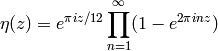
$\eta(z) = e^{\pi i z / 12} \prod_{n=1}^{\infty} (1 - e^{2\pi inz})$

EXAMPLES: We compute a few values of eta:

sage: CDF(0,1).eta()
0.768225422326
sage: CDF(1,1).eta()
0.742048775837 + 0.19883137023*I
sage: CDF(25,1).eta()
0.742048775837 + 0.19883137023*I

Eta works even if the inputs are large.

sage: CDF(0,10^15).eta()
0
sage: CDF(10^15,0.1).eta()     # slightly random-ish arch dependent output
-0.121339721991 - 0.19619461894*I   

We compute a few values of eta, but with the fractional power of e omitted.

sage: CDF(0,1).eta(True)
0.998129069926

We compute eta to low precision directly from the definition.

sage: z = CDF(1,1); z.eta()
0.742048775837 + 0.19883137023*I
sage: i = CDF(0,1); pi = CDF(pi)
sage: exp(pi * i * z / 12) * prod([1-exp(2*pi*i*n*z) for n in range(1,10)])
0.742048775837 + 0.19883137023*I

The optional argument allows us to omit the fractional part:

sage: z = CDF(1,1)
sage: z.eta(omit_frac=True)
0.998129069926
sage: pi = CDF(pi)
sage: prod([1-exp(2*pi*i*n*z) for n in range(1,10)])      # slightly random-ish arch dependent output
0.998129069926 + 4.5908467128e-19*I  

We illustrate what happens when $z$ is not in the upper half plane.

sage: z = CDF(1)
sage: z.eta()
...
ValueError: value must be in the upper half plane

You can also use functional notation.

sage: z = CDF(1,1) ; eta(z)
0.742048775837 + 0.19883137023*I

exp()¶

This function returns the complex exponential of the complex number $z$ , $\exp(z)$ .

EXAMPLES:

sage: CDF(1,1).exp()
1.46869393992 + 2.28735528718*I

We numerically verify a famous identity to the precision of a double.

sage: z = CDF(0, 2*pi); z
6.28318530718*I
sage: exp(z)         # somewhat random-ish output depending on platform
1.0 - 2.44921270764e-16*I

gamma()¶

Return the Gamma function evaluated at this complex number.

EXAMPLES:

sage: CDF(5,0).gamma()
24.0
sage: CDF(1,1).gamma()
0.498015668118 - 0.154949828302*I
sage: CDF(0).gamma()
Infinity
sage: CDF(-1,0).gamma()
Infinity

gamma_inc(t)¶

Return the incomplete Gamma function evaluated at this complex number.

EXAMPLES:

sage: CDF(1,1).gamma_inc(CDF(2,3))
0.00209691486365 - 0.0599819136554*I
sage: CDF(1,1).gamma_inc(5)
-0.00137813093622 + 0.00651982002312*I
sage: CDF(2,0).gamma_inc(CDF(1,1))
0.707092096346 - 0.42035364096*I

imag()¶

Return the imaginary part of this complex double.

EXAMPLES:

sage: a = CDF(3,-2)
sage: a.imag()
-2.0
sage: a.imag_part()
-2.0

imag_part()¶

Return the imaginary part of this complex double.

EXAMPLES:

sage: a = CDF(3,-2)
sage: a.imag()
-2.0
sage: a.imag_part()
-2.0

is_square()¶

This function always returns true as $\CC$ is algebraically closed.

EXAMPLES:

sage: CDF(-1).is_square()
True

log(base=None)¶

This function returns the complex natural logarithm to the given base of the complex number $z$ , $\log(z)$ . The branch cut is the negative real axis.

INPUT:

base - default: e, the base of the natural logarithm

EXAMPLES:

sage: CDF(1,1).log()
0.34657359028 + 0.785398163397*I

This is the only example different from the GSL:

sage: CDF(0,0).log()
-infinity

log10()¶

This function returns the complex base-10 logarithm of the complex number $z$ , $\log_{10}(z)$ .

The branch cut is the negative real axis.

EXAMPLES:

sage: CDF(1,1).log10()
0.150514997832 + 0.34109408846*I

log_b(b)¶

This function returns the complex base- $b$ logarithm of the complex number $z$ , $\log_b(z)$ . This quantity is computed as the ratio $\log(z)/\log(b)$ .

The branch cut is the negative real axis.

EXAMPLES:

sage: CDF(1,1).log_b(10)
0.150514997832 + 0.34109408846*I

logabs()¶

This function returns the natural logarithm of the magnitude of the complex number $z$ , $\log|z|$ .

This allows for an accurate evaluation of $\log|z|$ when $|z|$ is close to $1$ . The direct evaluation of log(abs(z)) would lead to a loss of precision in this case.

EXAMPLES:

sage: CDF(1.1,0.1).logabs()
0.0994254293726
sage: log(abs(CDF(1.1,0.1)))
0.0994254293726

sage: log(abs(ComplexField(200)(1.1,0.1)))
0.099425429372582595066319157757531449594489450091985182495705

norm()¶

This function returns the squared magnitude of the complex number $z$ , $|z|^2$ .

EXAMPLES:

sage: CDF(2,3).norm()
13.0

nth_root(n, all=False)¶

The n-th root function.

INPUT:

all - bool (default: False); if True, return a list of all n-th roots.

EXAMPLES:

sage: a = CDF(125)
sage: a.nth_root(3)
5.0
sage: a = CDF(10, 2)
sage: [r^5 for r in a.nth_root(5, all=True)]
[10.0 + 2.0*I, 10.0 + 2.0*I, 10.0 + 2.0*I, 10.0 + 2.0*I, 10.0 + 2.0*I]
sage: abs(sum(a.nth_root(111, all=True))) # random but close to zero
6.00659385991e-14

parent()¶

Return the complex double field, which is the parent of self.

EXAMPLES:

sage: a = CDF(2,3)
sage: a.parent()
Complex Double Field
sage: parent(a)
Complex Double Field

prec()¶

Returns the precision of this number (to be more similar to ComplexNumber). Always returns 53.

EXAMPLES:

sage: CDF(0).prec()
53

real()¶

Return the real part of this complex double.

EXAMPLES:

sage: a = CDF(3,-2)
sage: a.real()
3.0
sage: a.real_part()
3.0

real_part()¶

Return the real part of this complex double.

EXAMPLES:

sage: a = CDF(3,-2)
sage: a.real()
3.0
sage: a.real_part()
3.0

sec()¶

This function returns the complex secant of the complex number $z$ , ${\rm sec}(z) = 1/\cos(z)$ .

EXAMPLES:

sage: CDF(1,1).sec()
0.498337030555 + 0.591083841721*I

sech()¶

This function returns the complex hyperbolic secant of the complex number $z$ , ${\rm sech}(z) = 1/{\rm cosh}(z)$ .

EXAMPLES:

sage: CDF(1,1).sech()
0.498337030555 - 0.591083841721*I

sin()¶

This function returns the complex sine of the complex number $z$ , $\sin(z) = (\exp(iz) - \exp(-iz))/(2i)$ .

EXAMPLES:

sage: CDF(1,1).sin()
1.29845758142 + 0.634963914785*I

sinh()¶

This function returns the complex hyperbolic sine of the complex number $z$ , $\sinh(z) = (\exp(z) - \exp(-z))/2$ .

EXAMPLES:

sage: CDF(1,1).sinh()
0.634963914785 + 1.29845758142*I

sqrt(all, **kwds=False)¶

The square root function.

INPUT:

all - bool (default: False); if True, return a list of all square roots.

If all is False, the branch cut is the negative real axis. The result always lies in the right half of the complex plane.

EXAMPLES: We compute several square roots.

sage: a = CDF(2,3)
sage: b = a.sqrt(); b
1.67414922804 + 0.89597747613*I
sage: b^2
2.0 + 3.0*I
sage: a^(1/2)
1.67414922804 + 0.89597747613*I

We compute the square root of -1.

sage: a = CDF(-1)
sage: a.sqrt()
1.0*I

We compute all square roots:

sage: CDF(-2).sqrt(all=True)
[1.41421356237*I, -1.41421356237*I]
sage: CDF(0).sqrt(all=True)
[0]

tan()¶

This function returns the complex tangent of the complex number z, $\tan(z) = \sin(z)/\cos(z)$ .

EXAMPLES:

sage: CDF(1,1).tan()
0.27175258532 + 1.08392332734*I

tanh()¶

This function returns the complex hyperbolic tangent of the complex number $z$ , $\tanh(z) = \sinh(z)/\cosh(z)$ .

EXAMPLES:

sage: CDF(1,1).tanh()
1.08392332734 + 0.27175258532*I

zeta()¶

Return the Riemann zeta function evaluated at this complex number.

EXAMPLES:

sage: z = CDF(1, 1)
sage: z.zeta()
0.582158059752 - 0.926848564331*I
sage: zeta(z)
0.582158059752 - 0.926848564331*I

sage.rings.complex_double.ComplexDoubleField()¶

Returns the field of double precision complex numbers.

EXAMPLE:

sage: ComplexDoubleField()
Complex Double Field
sage: ComplexDoubleField() is CDF
True

class sage.rings.complex_double.ComplexDoubleField_class¶

Bases: sage.rings.ring.Field

An approximation to the field of complex numbers using double precision floating point numbers. Answers derived from calculations in this approximation may differ from what they would be if those calculations were performed in the true field of complex numbers. This is due to the rounding errors inherent to finite precision calculations.

ALGORITHMS: Arithmetic is done using GSL (the GNU Scientific Library).

characteristic()¶

Return the characteristic of this complex double field, which is 0.

EXAMPLES:

sage: CDF.characteristic()
0

construction()¶

Returns the functorial construction of self, namely, algebraic closure of the real double field.

EXAMPLES:

sage: c, S = CDF.construction(); S
Real Double Field
sage: CDF == c(S)
True

gen(n=0)¶

Return the generator of the complex double field.

EXAMPLES:

sage: CDF.0
1.0*I
sage: CDF.gens()
(1.0*I,)

is_exact()¶

Returns whether or not this field is exact, which is always false.

EXAMPLE:

sage: CDF.is_exact()
False

ngens()¶

The number of generators of this complex field as an RR-algebra.

There is one generator, namely sqrt(-1).

EXAMPLES:

sage: CDF.ngens()
1

pi()¶

Returns pi as a double precision complex number.

EXAMPLES:

sage: CDF.pi()
3.14159265359

prec()¶

Return the precision of this complex double field (to be more similar to ComplexField). Always returns 53.

EXAMPLES:

sage: CDF.prec()
53

random_element(xmin=-1, xmax=1, ymin=-1, ymax=1)¶

Return a random element this complex double field with real and imaginary part bounded by xmin, xmax, ymin, ymax.

EXAMPLES:

sage: CDF.random_element()
-0.436810529675 + 0.736945423566*I
sage: CDF.random_element(-10,10,-10,10)
-7.08874026302 - 9.54135400334*I
sage: CDF.random_element(-10^20,10^20,-2,2)
-7.58765473764e+19 + 0.925549022839*I

real_double_field()¶

The real double field, which you may view as a subfield of this complex double field.

EXAMPLES:

sage: CDF.real_double_field()
Real Double Field

to_prec(prec)¶

Returns the complex field to the specified precision. As doubles have fixed precision, this will only return a complex double field if prec is exactly 53.

EXAMPLES:

sage: CDF.to_prec(53)
Complex Double Field
sage: CDF.to_prec(250)
Complex Field with 250 bits of precision

zeta(n=2)¶

Return a primitive $n$ -th root of unity in this CDF, for $n\ge1$ .

INPUT:

n - a positive integer (default: 2)

OUTPUT: a complex n-th root of unity.

EXAMPLES:

sage: CDF.zeta(7)
0.623489801859 + 0.781831482468*I
sage: CDF.zeta(1)
1.0     
sage: CDF.zeta()
-1.0
sage: CDF.zeta() == CDF.zeta(2)
True

sage: CDF.zeta(0.5)
...
ValueError: n must be a positive integer
sage: CDF.zeta(0)
...
ValueError: n must be a positive integer
sage: CDF.zeta(-1)
...
ValueError: n must be a positive integer

class sage.rings.complex_double.FloatToCDF¶

Bases: sage.categories.morphism.Morphism

Fast morphism from anything with a __float__ method to an RDF element.

EXAMPLES:

sage: f = CDF.coerce_map_from(ZZ); f
Native morphism:
  From: Integer Ring
  To:   Complex Double Field
sage: f(4)
4.0
sage: f = CDF.coerce_map_from(QQ); f
Native morphism:
  From: Rational Field
  To:   Complex Double Field
sage: f(1/2)
0.5
sage: f = CDF.coerce_map_from(int); f
Native morphism:
  From: Set of Python objects of type 'int'
  To:   Complex Double Field
sage: f(3r)
3.0
sage: f = CDF.coerce_map_from(float); f
Native morphism:
  From: Set of Python objects of type 'float'
  To:   Complex Double Field
sage: f(3.5)
3.5

sage.rings.complex_double.is_ComplexDoubleElement(x)¶

Return True if x is a is_ComplexDoubleElement.

EXAMPLES:

sage: from sage.rings.complex_double import is_ComplexDoubleElement
sage: is_ComplexDoubleElement(0)
False
sage: is_ComplexDoubleElement(CDF(0))
True

sage.rings.complex_double.is_ComplexDoubleField(x)¶

Return True if x is the complex double field.

EXAMPLE:

sage: from sage.rings.complex_double import is_ComplexDoubleField
sage: is_ComplexDoubleField(CDF)
True
sage: is_ComplexDoubleField(ComplexField(53))
False

Double Precision Complex Numbers¶

Previous topic

Next topic

This Page

Navigation

Double Precision Complex Numbers¶

Previous topic

Next topic

This Page

Quick search

Navigation