Power Series¶

Sage provides an implementation of dense and sparse power series over any Sage base ring.

AUTHORS:

William Stein
David Harvey (2006-09-11): added solve_linear_de() method
Robert Bradshaw (2007-04): sqrt, rmul, lmul, shifting
Robert Bradshaw (2007-04): Cython version

EXAMPLE:

sage: R.<x> = PowerSeriesRing(ZZ)
sage: R([1,2,3])
1 + 2*x + 3*x^2
sage: R([1,2,3], 10)
1 + 2*x + 3*x^2 + O(x^10)    
sage: f = 1 + 2*x - 3*x^3 + O(x^4); f
1 + 2*x - 3*x^3 + O(x^4)
sage: f^10
1 + 20*x + 180*x^2 + 930*x^3 + O(x^4)
sage: g = 1/f; g
1 - 2*x + 4*x^2 - 5*x^3 + O(x^4)
sage: g * f
1 + O(x^4)

In Python (as opposed to Sage) create the power series ring and its generator as follows:

sage: R, x = objgen(PowerSeriesRing(ZZ, 'x'))
sage: parent(x)
Power Series Ring in x over Integer Ring

EXAMPLE:

This example illustrates that coercion for power series rings is consistent with coercion for polynomial rings.

sage: poly_ring1.<gen1> = PolynomialRing(QQ)
sage: poly_ring2.<gen2> = PolynomialRing(QQ)
sage: huge_ring.<x> = PolynomialRing(poly_ring1)

The generator of the first ring gets coerced in as itself, since it is the base ring.

sage: huge_ring(gen1)
gen1

The generator of the second ring gets mapped via the natural map sending one generator to the other.

sage: huge_ring(gen2)
x

With power series the behavior is the same.

sage: power_ring1.<gen1> = PowerSeriesRing(QQ)
sage: power_ring2.<gen2> = PowerSeriesRing(QQ)
sage: huge_power_ring.<x> = PowerSeriesRing(power_ring1)
sage: huge_power_ring(gen1)
gen1
sage: huge_power_ring(gen2)
x 

TODO: Rewrite valuation so it is carried along after any calculation, so in almost all cases f.valuation() is instant. Also, if you add f and g and their valuations are the same, note that we only have to look at terms at positions = f.valuation().

class sage.rings.power_series_ring_element.PowerSeries¶

Bases: sage.structure.element.AlgebraElement

A power series.

O(prec)¶: Return this series plus $O(x^\text{prec})$ . Does not change self.

V(n)¶: If $f = \sum a_m x^m$ , then this function returns $\sum a_m x^{nm}$ .

add_bigoh(prec)¶

Returns the power series of precision at most prec got by adding $O(q^\text{prec})$ to f, where q is the variable.

EXAMPLES:

sage: R.<A> = RDF[[]]
sage: f = (1+A+O(A^5))^5; f
1.0 + 5.0*A + 10.0*A^2 + 10.0*A^3 + 5.0*A^4 + O(A^5)
sage: f.add_bigoh(3)
1.0 + 5.0*A + 10.0*A^2 + O(A^3)
sage: f.add_bigoh(5)
1.0 + 5.0*A + 10.0*A^2 + 10.0*A^3 + 5.0*A^4 + O(A^5)

base_extend(R)¶

Return a copy of this power series but with coefficients in R.

The following coercion uses base_extend implicitly:

sage: R.<t> = ZZ[['t']]
sage: (t - t^2) * Mod(1, 3)
t + 2*t^2

base_ring()¶

Return the base ring that this power series is defined over.

EXAMPLES:

sage: R.<t> = GF(49,'alpha')[[]]
sage: (t^2 + O(t^3)).base_ring()
Finite Field in alpha of size 7^2

change_ring(R)¶

Change if possible the coefficients of self to lie in R.

EXAMPLES:

sage: R.<T> = QQ[[]]; R
Power Series Ring in T over Rational Field
sage: f = 1 - 1/2*T + 1/3*T^2 + O(T^3)
sage: f.base_extend(GF(5))
...
TypeError: no base extension defined
sage: f.change_ring(GF(5))
1 + 2*T + 2*T^2 + O(T^3)
sage: f.change_ring(GF(3))
...
ZeroDivisionError: Inverse does not exist.        

We can only change ring if there is a __call__ coercion defined. The following succeeds because ZZ(K(4)) is defined.

sage: K.<a> = NumberField(cyclotomic_polynomial(3), 'a')
sage: R.<t> = K[['t']]
sage: (4*t).change_ring(ZZ)
4*t

This does not succeed because ZZ(K(a+1)) is not defined.

sage: K.<a> = NumberField(cyclotomic_polynomial(3), 'a')
sage: R.<t> = K[['t']]
sage: ((a+1)*t).change_ring(ZZ)
...
TypeError: Unable to coerce a + 1 to an integer

coefficients()¶

Return the nonzero coefficients of self.

EXAMPLES:

sage: R.<t> = PowerSeriesRing(QQ)
sage: f = t + t^2 - 10/3*t^3
sage: f.coefficients()
[1, 1, -10/3]

common_prec(f)¶

Returns minimum precision of $f$ and self.

EXAMPLES:

sage: R.<t> = PowerSeriesRing(QQ)

sage: f = t + t^2 + O(t^3)
sage: g = t + t^3 + t^4 + O(t^4)
sage: f.common_prec(g)
3
sage: g.common_prec(f)
3

sage: f = t + t^2 + O(t^3)
sage: g = t^2
sage: f.common_prec(g)
3
sage: g.common_prec(f)
3

sage: f = t + t^2
sage: f = t^2
sage: f.common_prec(g)
+Infinity

degree()¶

Return the degree of this power series, which is by definition the degree of the underlying polynomial.

EXAMPLES:

sage: R.<t> = PowerSeriesRing(QQ, sparse=True)
sage: f = t^100000 + O(t^10000000)
sage: f.degree()
100000

derivative(*args)¶

The formal derivative of this power series, with respect to variables supplied in args.

Multiple variables and iteration counts may be supplied; see documentation for the global derivative() function for more details.

See also

_derivative()

EXAMPLES:

sage: R.<x> = PowerSeriesRing(QQ)
sage: g = -x + x^2/2 - x^4 + O(x^6)
sage: g.derivative()
-1 + x - 4*x^3 + O(x^5)
sage: g.derivative(x)
-1 + x - 4*x^3 + O(x^5)
sage: g.derivative(x, x)
1 - 12*x^2 + O(x^4)
sage: g.derivative(x, 2)
1 - 12*x^2 + O(x^4)

egf()¶

Returns the exponential generating function associated to self.

This function is known as serlaplace in GP/PARI.

EXAMPLES:

sage: R.<t> = PowerSeriesRing(QQ)
sage: f = t + t^2 + 2*t^3
sage: f.egf()
t + 1/2*t^2 + 1/3*t^3

exp(prec=None)¶

Returns exp of this power series to the indicated precision.

INPUT:

prec - integer; default is self.parent().default_prec

ALGORITHM: See PowerSeries.solve_linear_de().

Note

Screwy things can happen if the coefficient ring is not a field of characteristic zero. See PowerSeries.solve_linear_de().

AUTHORS:

David Harvey (2006-09-08): rewrote to use simplest possible “lazy” algorithm.
David Harvey (2006-09-10): rewrote to use divide-and-conquer strategy.
David Harvey (2006-09-11): factored functionality out to solve_linear_de().
Sourav Sen Gupta, David Harvey (2008-11): handle constant term

EXAMPLES:

sage: R.<t> = PowerSeriesRing(QQ, default_prec=10)

Check that $\exp(t)$ is, well, $\exp(t)$ :

sage: (t + O(t^10)).exp()
1 + t + 1/2*t^2 + 1/6*t^3 + 1/24*t^4 + 1/120*t^5 + 1/720*t^6 + 1/5040*t^7 + 1/40320*t^8 + 1/362880*t^9 + O(t^10)

Check that $\exp(\log(1+t))$ is $1+t$ :

sage: (sum([-(-t)^n/n for n in range(1, 10)]) + O(t^10)).exp()
1 + t + O(t^10)

Check that $\exp(2t + t^2 - t^5)$ is whatever it is:

sage: (2*t + t^2 - t^5 + O(t^10)).exp()
1 + 2*t + 3*t^2 + 10/3*t^3 + 19/6*t^4 + 8/5*t^5 - 7/90*t^6 - 538/315*t^7 - 425/168*t^8 - 30629/11340*t^9 + O(t^10)

Check requesting lower precision:

sage: (t + t^2 - t^5 + O(t^10)).exp(5)
1 + t + 3/2*t^2 + 7/6*t^3 + 25/24*t^4 + O(t^5)

Can’t get more precision than the input:

sage: (t + t^2 + O(t^3)).exp(10)
1 + t + 3/2*t^2 + O(t^3)

Check some boundary cases:

sage: (t + O(t^2)).exp(1)
1 + O(t)
sage: (t + O(t^2)).exp(0)
O(t^0)

Handle nonzero constant term (fixes trac #4477):

sage: R.<x> = PowerSeriesRing(RR)
sage: (1 + x + x^2 + O(x^3)).exp()
2.71828182845905 + 2.71828182845905*x + 4.07742274268857*x^2 + O(x^3)

sage: R.<x> = PowerSeriesRing(ZZ)
sage: (1 + x + O(x^2)).exp()
...
ArithmeticError: exponential of constant term does not belong to coefficient ring (consider working in a larger ring)           

sage: R.<x> = PowerSeriesRing(GF(5))
sage: (1 + x + O(x^2)).exp()
...
ArithmeticError: constant term of power series does not support exponentiation

exponents()¶

Return the exponents appearing in self with nonzero coefficients.

EXAMPLES:

sage: R.<t> = PowerSeriesRing(QQ)
sage: f = t + t^2 - 10/3*t^3
sage: f.exponents()
[1, 2, 3]

is_dense()¶

EXAMPLES:

sage: R.<t> = PowerSeriesRing(ZZ)
sage: t.is_dense()
True
sage: R.<t> = PowerSeriesRing(ZZ, sparse=True)
sage: t.is_dense()
False

is_gen()¶

Returns True if this the generator (the variable) of the power series ring.

EXAMPLES:

sage: R.<t> = QQ[[]]
sage: t.is_gen()
True
sage: (1 + 2*t).is_gen()
False

Note that this only returns true on the actual generator, not on something that happens to be equal to it.

sage: (1*t).is_gen()
False
sage: 1*t == t
True

is_sparse()¶

EXAMPLES:

sage: R.<t> = PowerSeriesRing(ZZ)
sage: t.is_sparse()
False        
sage: R.<t> = PowerSeriesRing(ZZ, sparse=True)
sage: t.is_sparse()
True

is_square()¶

Returns True if this function has a square root in this ring, e.g. there is an element $y$ in self.parent() such that $y^2 = ``self``$ .

ALGORITHM: If the base ring is a field, this is true whenever the power series has even valuation and the leading coefficient is a perfect square.

For an integral domain, it attempts the square root in the fraction field and tests whether or not the result lies in the original ring.

EXAMPLES:

sage: K.<t> = PowerSeriesRing(QQ, 't', 5)
sage: (1+t).is_square()
True
sage: (2+t).is_square()
False
sage: (2+t.change_ring(RR)).is_square()
True
sage: t.is_square()
False
sage: K.<t> = PowerSeriesRing(ZZ, 't', 5)
sage: (1+t).is_square()
False
sage: f = (1+t)^100
sage: f.is_square()
True

is_unit()¶

Returns whether this power series is invertible, which is the case precisely when the constant term is invertible.

EXAMPLES:

sage: R.<t> = PowerSeriesRing(ZZ)
sage: (-1 + t - t^5).is_unit()
True
sage: (3 + t - t^5).is_unit()
False

AUTHORS:

David Harvey (2006-09-03)

laurent_series()¶

Return the Laurent series associated to this power series, i.e., this series considered as a Laurent series.

EXAMPLES:

sage: k.<w> = QQ[[]]
sage: f = 1+17*w+15*w^3+O(w^5)
sage: parent(f)
Power Series Ring in w over Rational Field
sage: g = f.laurent_series(); g
1 + 17*w + 15*w^3 + O(w^5)

list()¶

ogf()¶

Returns the ordinary generating function associated to self.

This function is known as serlaplace in GP/PARI.

EXAMPLES:

sage: R.<t> = PowerSeriesRing(QQ)
sage: f = t + t^2/factorial(2) + 2*t^3/factorial(3)
sage: f.ogf()
t + t^2 + 2*t^3

padded_list(n=None)¶

Return a list of coefficients of self up to (but not including) $q^n$ .

Includes 0’s in the list on the right so that the list has length $n$ .

INPUT:

n - (optional) an integer that is at least 0. If n is not given, it will be taken to be the precision of self, unless this is +Infinity, in which case we just return self.list().

EXAMPLES:

sage: R.<q> = PowerSeriesRing(QQ)
sage: f = 1 - 17*q + 13*q^2 + 10*q^4 + O(q^7)
sage: f.list()
[1, -17, 13, 0, 10]
sage: f.padded_list(7)
[1, -17, 13, 0, 10, 0, 0]
sage: f.padded_list(10)
[1, -17, 13, 0, 10, 0, 0, 0, 0, 0]
sage: f.padded_list(3)
[1, -17, 13]
sage: f.padded_list()
[1, -17, 13, 0, 10, 0, 0]
sage: g = 1 - 17*q + 13*q^2 + 10*q^4
sage: g.list()
[1, -17, 13, 0, 10]
sage: g.padded_list()
[1, -17, 13, 0, 10]
sage: g.padded_list(10)
[1, -17, 13, 0, 10, 0, 0, 0, 0, 0]

polynomial()¶

prec()¶

The precision of $...+O(x^r)$ is by definition $r$ .

EXAMPLES:

sage: R.<t> = ZZ[[]]
sage: (t^2 + O(t^3)).prec()
3
sage: (1 - t^2 + O(t^100)).prec()
100

shift(n)¶

Returns this power series multiplied by the power $t^n$ . If $n$ is negative, terms below $t^n$ will be discarded. Does not change this power series.

Note

Despite the fact that higher order terms are printed to the right in a power series, right shifting decreases the powers of $t$ , while left shifting increases them. This is to be consistent with polynomials, integers, etc.

EXAMPLES:

sage: R.<t> = PowerSeriesRing(QQ['y'], 't', 5)
sage: f = ~(1+t); f
1 - t + t^2 - t^3 + t^4 + O(t^5)
sage: f.shift(3)
t^3 - t^4 + t^5 - t^6 + t^7 + O(t^8)
sage: f >> 2
1 - t + t^2 + O(t^3)
sage: f << 10
t^10 - t^11 + t^12 - t^13 + t^14 + O(t^15)
sage: t << 29
t^30

AUTHORS:

Robert Bradshaw (2007-04-18)

solve_linear_de(prec=' infinity', b=None, f0=None)¶

Obtains a power series solution to an inhomogeneous linear differential equation of the form:

$f'(t) = a(t) f(t) + b(t).$

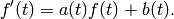
INPUT:

self - the power series $a(t)$
b - the power series $b(t)$ (default is zero)
f0 - the constant term of $f$ (“initial condition”) (default is 1)
prec - desired precision of result (this will be reduced if either a or b have less precision available)

OUTPUT: the power series f, to indicated precision

ALGORITHM: A divide-and-conquer strategy; see the source code. Running time is approximately $M(n) \log n$ , where $M(n)$ is the time required for a polynomial multiplication of length $n$ over the coefficient ring. (If you’re working over something like RationalField(), running time analysis can be a little complicated because the coefficients tend to explode.)

Note

If the coefficient ring is a field of characteristic zero, then the solution will exist and is unique.
For other coefficient rings, things are more complicated. A solution may not exist, and if it does it may not be unique. Generally, by the time the nth term has been computed, the algorithm will have attempted divisions by $n!$ in the coefficient ring. So if your coefficient ring has enough ‘precision’, and if your coefficient ring can perform divisions even when the answer is not unique, and if you know in advance that a solution exists, then this function will find a solution (otherwise it will probably crash).

AUTHORS:

David Harvey (2006-09-11): factored functionality out from exp() function, cleaned up precision tests a bit

EXAMPLES:

sage: R.<t> = PowerSeriesRing(QQ, default_prec=10)

sage: a = 2 - 3*t + 4*t^2 + O(t^10)
sage: b = 3 - 4*t^2 + O(t^7)
sage: f = a.solve_linear_de(prec=5, b=b, f0=3/5)
sage: f
 3/5 + 21/5*t + 33/10*t^2 - 38/15*t^3 + 11/24*t^4 + O(t^5)
sage: f.derivative() - a*f - b
 O(t^4)

sage: a = 2 - 3*t + 4*t^2
sage: b = b = 3 - 4*t^2
sage: f = a.solve_linear_de(b=b, f0=3/5)
...
ValueError: cannot solve differential equation to infinite precision

sage: a.solve_linear_de(prec=5, b=b, f0=3/5)
 3/5 + 21/5*t + 33/10*t^2 - 38/15*t^3 + 11/24*t^4 + O(t^5)

sqrt(prec=None, extend=False, all=False, name=None)¶

INPUT:

prec - integer (default: None): if not None and the series has infinite precision, truncates series at precision prec.

extend - bool (default: False); if True, return a square root in an extension ring, if necessary. Otherwise, raise a ValueError if the square is not in the base power series ring. For example, if extend is True the square root of a power series with odd degree leading coefficient is defined as an element of a formal extension ring.

name - if extend is True, you must also specify the print name of the formal square root.

all - bool (default: False); if True, return all square roots of self, instead of just one.

ALGORITHM: Newton’s method

$x_{i+1} = \frac{1}{2}( x_i + self/x_i )$

EXAMPLES:
sage: K.<t> = PowerSeriesRing(QQ, 't', 5)
sage: sqrt(t^2)
t
sage: sqrt(1+t)
1 + 1/2*t - 1/8*t^2 + 1/16*t^3 - 5/128*t^4 + O(t^5)
sage: sqrt(4+t)
2 + 1/4*t - 1/64*t^2 + 1/512*t^3 - 5/16384*t^4 + O(t^5)
sage: u = sqrt(2+t, prec=2, extend=True, name = 'alpha'); u
alpha
sage: u^2
2 + t
sage: u.parent()
Univariate Quotient Polynomial Ring in alpha over Power Series Ring in t over Rational Field with modulus x^2 - 2 - t
sage: K.<t> = PowerSeriesRing(QQ, 't', 50)
sage: sqrt(1+2*t+t^2)
1 + t
sage: sqrt(t^2 +2*t^4 + t^6)
t + t^3
sage: sqrt(1 + t + t^2 + 7*t^3)^2
1 + t + t^2 + 7*t^3 + O(t^50)
sage: sqrt(K(0))
0
sage: sqrt(t^2)
t
sage: K.<t> = PowerSeriesRing(CDF, 5)
sage: v = sqrt(-1 + t + t^3, all=True); v
[1.0*I - 0.5*I*t - 0.125*I*t^2 - 0.5625*I*t^3 - 0.2890625*I*t^4 + O(t^5),
 -1.0*I + 0.5*I*t + 0.125*I*t^2 + 0.5625*I*t^3 + 0.2890625*I*t^4 + O(t^5)]
sage: [a^2 for a in v]
[-1.0 + 1.0*t + 1.0*t^3 + O(t^5), -1.0 + 1.0*t + 1.0*t^3 + O(t^5)]
A formal square root:
sage: K.<t> = PowerSeriesRing(QQ, 5)
sage: f = 2*t + t^3 + O(t^4)
sage: s = f.sqrt(extend=True, name='sqrtf'); s
sqrtf
sage: s^2
2*t + t^3 + O(t^4)
sage: parent(s)
Univariate Quotient Polynomial Ring in sqrtf over Power Series Ring in t over Rational Field with modulus x^2 - 2*t - t^3 + O(t^4)
TESTS:
sage: R.<x> = QQ[[]]
sage: (x^10/2).sqrt()
...
ValueError: unable to take the square root of 1/2
AUTHORS:

Robert Bradshaw

William Stein

square_root()¶

Return the square root of self in this ring. If this cannot be done then an error will be raised.

This function succeeds if and only if self.is_square()

EXAMPLES:

sage: K.<t> = PowerSeriesRing(QQ, 't', 5)
sage: (1+t).square_root()
1 + 1/2*t - 1/8*t^2 + 1/16*t^3 - 5/128*t^4 + O(t^5)
sage: (2+t).square_root()
...
ValueError: Square root does not live in this ring.
sage: (2+t.change_ring(RR)).square_root()
1.41421356237309 + 0.353553390593274*t - 0.0441941738241592*t^2 + 0.0110485434560398*t^3 - 0.00345266983001244*t^4 + O(t^5)
sage: t.square_root()
...
ValueError: Square root not defined for power series of odd valuation.
sage: K.<t> = PowerSeriesRing(ZZ, 't', 5)
sage: f = (1+t)^20
sage: f.square_root()
1 + 10*t + 45*t^2 + 120*t^3 + 210*t^4 + O(t^5)
sage: f = 1+t
sage: f.square_root()
...
ValueError: Square root does not live in this ring.

AUTHORS:

Robert Bradshaw

truncate(prec='infinity')¶

The polynomial obtained from power series by truncation.

EXAMPLES:

sage: R.<I> = GF(2)[[]]
sage: f = 1/(1+I+O(I^8)); f
1 + I + I^2 + I^3 + I^4 + I^5 + I^6 + I^7 + O(I^8)
sage: f.truncate(5)
I^4 + I^3 + I^2 + I + 1

valuation()¶

Return the valuation of this power series.

This is equal to the valuation of the underlying polynomial.

EXAMPLES: Sparse examples:

sage: R.<t> = PowerSeriesRing(QQ, sparse=True)
sage: f = t^100000 + O(t^10000000)
sage: f.valuation()
100000
sage: R(0).valuation()
+Infinity

Dense examples:

sage: R.<t> = PowerSeriesRing(ZZ)
sage: f = 17*t^100 +O(t^110)
sage: f.valuation()
100
sage: t.valuation()
1

valuation_zero_part()¶

Factor self as as $q^n \cdot (a_0 + a_1 q + \cdots)$ with $a_0$ nonzero. Then this function returns $a_0 + a_1 q + \cdots$ .

Note

This valuation zero part need not be a unit if, e.g., $a_0$ is not invertible in the base ring.

EXAMPLES:

sage: R.<t> = PowerSeriesRing(QQ)
sage: ((1/3)*t^5*(17-2/3*t^3)).valuation_zero_part()
17/3 - 2/9*t^3        

In this example the valuation 0 part is not a unit:

sage: R.<t> = PowerSeriesRing(ZZ, sparse=True)
sage: u = (-2*t^5*(17-t^3)).valuation_zero_part(); u
-34 + 2*t^3
sage: u.is_unit()
False
sage: u.valuation()
0

variable()¶

EXAMPLES:

sage: R.<x> = PowerSeriesRing(Rationals())
sage: f = x^2 + 3*x^4 + O(x^7)
sage: f.variable()
'x'

AUTHORS:

David Harvey (2006-08-08)

sage.rings.power_series_ring_element.is_PowerSeries(x)¶

sage.rings.power_series_ring_element.make_element_from_parent_v0(parent, *args)¶

sage.rings.power_series_ring_element.make_powerseries_poly_v0(parent, f, prec, is_gen)¶

Power Series¶

Previous topic

Next topic

This Page

Navigation

Power Series¶

Previous topic

Next topic

This Page

Quick search

Navigation