Univariate Polynomial Rings¶

Sage implements sparse and dense polynomials over commutative and non-commutative rings. In the non-commutative case, the polynomial variable commutes with the elements of the base ring.

AUTHOR:

William Stein
Kiran Kedlaya (2006-02-13): added macaulay2 option
Martin Albrecht (2006-08-25): removed it again as it isn’t needed anymore

EXAMPLES: Creating a polynomial ring injects the variable into the interpreter namespace:

sage: z = QQ['z'].0
sage: (z^3 + z - 1)^3
z^9 + 3*z^7 - 3*z^6 + 3*z^5 - 6*z^4 + 4*z^3 - 3*z^2 + 3*z - 1

Saving and loading of polynomial rings works:

sage: loads(dumps(QQ['x'])) == QQ['x']
True
sage: k = PolynomialRing(QQ['x'],'y'); loads(dumps(k))==k
True    
sage: k = PolynomialRing(ZZ,'y'); loads(dumps(k)) == k
True
sage: k = PolynomialRing(ZZ,'y', sparse=True); loads(dumps(k))
Sparse Univariate Polynomial Ring in y over Integer Ring

The rings of sparse and dense polynomials in the same variable are canonically isomorphic:

sage: PolynomialRing(ZZ,'y', sparse=True) == PolynomialRing(ZZ,'y')
True

sage: QQ['y'] < QQ['x']
False
sage: QQ['y'] < QQ['z']
True

We create a polynomial ring over a quaternion algebra:

sage: A.<i,j,k> = QuaternionAlgebra(QQ, -1,-1)
sage: R.<w> = PolynomialRing(A,sparse=True)
sage: f = w^3 + (i+j)*w + 1
sage: f
w^3 + (i + j)*w + 1
sage: f^2
w^6 + (2*i + 2*j)*w^4 + 2*w^3 - 2*w^2 + (2*i + 2*j)*w + 1
sage: f = w + i ; g = w + j
sage: f * g
w^2 + (i + j)*w + k
sage: g * f
w^2 + (i + j)*w - k

TESTS:

sage: K.<x>=FractionField(QQ['x'])
sage: V.<z> = K[]
sage: x+z
z + x

These may change over time:

sage: type(ZZ['x'].0)
<type 'sage.rings.polynomial.polynomial_integer_dense_flint.Polynomial_integer_dense_flint'>
sage: type(QQ['x'].0)
<class 'sage.rings.polynomial.polynomial_element_generic.Polynomial_rational_dense'>
sage: type(RR['x'].0)
<type 'sage.rings.polynomial.polynomial_real_mpfr_dense.PolynomialRealDense'>
sage: type(Integers(4)['x'].0)
<type 'sage.rings.polynomial.polynomial_zmod_flint.Polynomial_zmod_flint'>
sage: type(Integers(5*2^100)['x'].0)
<type 'sage.rings.polynomial.polynomial_modn_dense_ntl.Polynomial_dense_modn_ntl_ZZ'>
sage: type(CC['x'].0)
<class 'sage.rings.polynomial.polynomial_element_generic.Polynomial_generic_dense_field'>
sage: type(CC['t']['x'].0)
<type 'sage.rings.polynomial.polynomial_element.Polynomial_generic_dense'>

class sage.rings.polynomial.polynomial_ring.PolynomialRing_commutative(base_ring, name=None, sparse=False, element_class=None)¶

Bases: sage.rings.polynomial.polynomial_ring.PolynomialRing_general, sage.rings.ring.CommutativeAlgebra

Univariate polynomial ring over a commutative ring.

quotient_by_principal_ideal(f, names=None)¶

Return the quotient of this polynomial ring by the principal ideal (generated by) $f$ .

INPUT:

f - either a polynomial in self, or a principal ideal of self.

EXAMPLES:

sage: R.<x> = QQ[]
sage: I = (x^2-1)*R
sage: R.quotient_by_principal_ideal(I)
Univariate Quotient Polynomial Ring in xbar over Rational Field with modulus x^2 - 1

The same example, using the polynomial instead of the ideal, and customizing the variable name:

sage: R.<x> = QQ[]
sage: R.quotient_by_principal_ideal(x^2-1, names=('foo',))
Univariate Quotient Polynomial Ring in foo over Rational Field with modulus x^2 - 1

class sage.rings.polynomial.polynomial_ring.PolynomialRing_dense_mod_n(base_ring, name=None, element_class=None, implementation=None)¶

Bases: sage.rings.polynomial.polynomial_ring.PolynomialRing_commutative

modulus()¶

EXAMPLES:

sage: R.<x> = Zmod(15)[]
sage: R.modulus()
15

class sage.rings.polynomial.polynomial_ring.PolynomialRing_dense_mod_p(base_ring, name='x', implementation=None)¶: Bases: sage.rings.polynomial.polynomial_ring.PolynomialRing_field, sage.rings.polynomial.polynomial_ring.PolynomialRing_dense_mod_n, sage.rings.polynomial.polynomial_singular_interface.PolynomialRing_singular_repr

class sage.rings.polynomial.polynomial_ring.PolynomialRing_dense_padic_field_capped_relative(base_ring, name=None, element_class=None)¶: Bases: sage.rings.polynomial.polynomial_ring.PolynomialRing_dense_padic_field_generic

class sage.rings.polynomial.polynomial_ring.PolynomialRing_dense_padic_field_generic(base_ring, name='x', sparse=False, element_class=None, implementation=None)¶: Bases: sage.rings.polynomial.polynomial_ring.PolynomialRing_field

class sage.rings.polynomial.polynomial_ring.PolynomialRing_dense_padic_field_lazy(base_ring, name=None, element_class=None)¶: Bases: sage.rings.polynomial.polynomial_ring.PolynomialRing_dense_padic_field_generic

class sage.rings.polynomial.polynomial_ring.PolynomialRing_dense_padic_ring_capped_absolute(base_ring, name=None, element_class=None)¶: Bases: sage.rings.polynomial.polynomial_ring.PolynomialRing_dense_padic_ring_generic

class sage.rings.polynomial.polynomial_ring.PolynomialRing_dense_padic_ring_capped_relative(base_ring, name=None, element_class=None)¶: Bases: sage.rings.polynomial.polynomial_ring.PolynomialRing_dense_padic_ring_generic

class sage.rings.polynomial.polynomial_ring.PolynomialRing_dense_padic_ring_fixed_mod(base_ring, name=None, element_class=None)¶: Bases: sage.rings.polynomial.polynomial_ring.PolynomialRing_dense_padic_ring_generic

class sage.rings.polynomial.polynomial_ring.PolynomialRing_dense_padic_ring_generic(base_ring, name='x', sparse=False, implementation=None, element_class=None)¶: Bases: sage.rings.polynomial.polynomial_ring.PolynomialRing_integral_domain

class sage.rings.polynomial.polynomial_ring.PolynomialRing_dense_padic_ring_lazy(base_ring, name=None, element_class=None)¶: Bases: sage.rings.polynomial.polynomial_ring.PolynomialRing_dense_padic_ring_generic

class sage.rings.polynomial.polynomial_ring.PolynomialRing_field(base_ring, name='x', sparse=False, element_class=None, implementation=None)¶

Bases: sage.rings.polynomial.polynomial_ring.PolynomialRing_integral_domain, sage.rings.polynomial.polynomial_singular_interface.PolynomialRing_singular_repr, sage.rings.ring.PrincipalIdealDomain

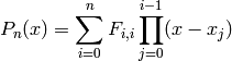
divided_difference(points, full_table=False)¶

Return the Newton divided-difference coefficients of the $n$ -th Lagrange interpolation polynomial of points.

If points are $n+1$ distinct points $(x_0, f(x_0)), (x_1, f(x_1)), \dots, (x_n, f(x_n))$ , then $P_n(x)$ is the $n$ -th Lagrange interpolation polynomial of $f(x)$ that passes through the points $(x_i, f(x_i))$ . This method returns the coefficients $F_{i,i}$ such that

$P_n(x) = \sum_{i=0}^n F_{i,i} \prod_{j=0}^{i-1} (x - x_j)$

INPUT:

points – a list of tuples $(x_0, f(x_0)), (x_1, f(x_1)), \dots, (x_n, f(x_n))$ where each $x_i \neq x_j$ for $i \neq j$
full_table – (default: False) if True then return the full divided-difference table; if False then only return entries along the main diagonal. The entries along the main diagonal are the Newton divided-difference coefficients $F_{i,i}$ .

OUTPUT:

The Newton divided-difference coefficients of the $n$ -th Lagrange interpolation polynomial that passes through the points in points.

EXAMPLES:

Only return the divided-difference coefficients $F_{i,i}$ . This example is taken from Example 1, p.121 of [BF05]:

sage: points = [(1.0, 0.7651977), (1.3, 0.6200860), (1.6, 0.4554022), (1.9, 0.2818186), (2.2, 0.1103623)]
sage: R = PolynomialRing(QQ, "x")
sage: R.divided_difference(points)
<BLANKLINE>
[0.765197700000000,
-0.483705666666666,
-0.108733888888889,
0.0658783950617283,
0.00182510288066044]

Now return the full divided-difference table:

sage: points = [(1.0, 0.7651977), (1.3, 0.6200860), (1.6, 0.4554022), (1.9, 0.2818186), (2.2, 0.1103623)]
sage: R = PolynomialRing(QQ, "x")
sage: R.divided_difference(points, full_table=True)
<BLANKLINE>
[[0.765197700000000],
[0.620086000000000, -0.483705666666666],
[0.455402200000000, -0.548946000000000, -0.108733888888889],
[0.281818600000000,
-0.578612000000000,
-0.0494433333333339,
0.0658783950617283],
[0.110362300000000,
-0.571520999999999,
0.0118183333333349,
0.0680685185185209,
0.00182510288066044]]

The following example is taken from Example 4.12, p.225 of [MF99]:

sage: points = [(1, -3), (2, 0), (3, 15), (4, 48), (5, 105), (6, 192)]
sage: R = PolynomialRing(RR, "x")
sage: R.divided_difference(points)
[-3, 3, 6, 1, 0, 0]
sage: R.divided_difference(points, full_table=True)
<BLANKLINE>
[[-3],
[0, 3],
[15, 15, 6],
[48, 33, 9, 1],
[105, 57, 12, 1, 0],
[192, 87, 15, 1, 0, 0]]

REFERENCES:

[MF99]

J.H. Mathews and K.D. Fink. Numerical Methods Using MATLAB. 3rd edition, Prentice-Hall, 1999.

lagrange_polynomial(points, algorithm='divided_difference', previous_row=None)¶

Return the Lagrange interpolation polynomial in self associated to the given list of points.

Given a list of points, i.e. tuples of elements of self‘s base ring, this function returns the interpolation polynomial in the Lagrange form.

INPUT:

points – a list of tuples representing points through which the polynomial returned by this function must pass.
algorithm – (default: 'divided_difference') the available values for this option are 'divided_difference' and neville.
- If algorithm='divided_difference' then use the method of divided difference.
- If algorithm='neville' then adapt Neville’s method as described on page 144 of [BF05] to recursively generate the Lagrange interpolation polynomial. Neville’s method generates a table of approximating polynomials, where the last row of that table contains the $n$ -th Lagrange interpolation polynomial. The adaptation implemented by this method is to only generate the last row of this table, instead of the full table itself. Generating the full table can be memory inefficient.
previous_row – (default: None) This option is only relevant if used together with algorithm='neville'. If provided, this should be the last row of the table resulting from a previous use of Neville’s method. If such a row is passed in, then points should consist of both previous and new interpolating points. Neville’s method will then use that last row and the interpolating points to generate a new row which contains a better Lagrange interpolation polynomial.

EXAMPLES:

By default, we use the method of divided-difference:

sage: R = PolynomialRing(QQ, 'x')
sage: f = R.lagrange_polynomial([(0,1),(2,2),(3,-2),(-4,9)]); f
-23/84*x^3 - 11/84*x^2 + 13/7*x + 1
sage: f(0)
1
sage: f(2)
2
sage: f(3)
-2
sage: f(-4)
9
sage: R = PolynomialRing(GF(2**3,'a'), 'x')
sage: a = R.base_ring().gen()
sage: f = R.lagrange_polynomial([(a^2+a,a),(a,1),(a^2,a^2+a+1)]); f
a^2*x^2 + a^2*x + a^2
sage: f(a^2+a)
a
sage: f(a)
1
sage: f(a^2)
a^2 + a + 1

Now use a memory efficient version of Neville’s method:

sage: R = PolynomialRing(QQ, 'x')
sage: R.lagrange_polynomial([(0,1),(2,2),(3,-2),(-4,9)], algorithm="neville")
<BLANKLINE>
[9,
-11/7*x + 19/7,
-17/42*x^2 - 83/42*x + 53/7,
-23/84*x^3 - 11/84*x^2 + 13/7*x + 1]
sage: R = PolynomialRing(GF(2**3,'a'), 'x')
sage: a = R.base_ring().gen()
sage: R.lagrange_polynomial([(a^2+a,a),(a,1),(a^2,a^2+a+1)], algorithm="neville")                                                                         
[a^2 + a + 1, x + a + 1, a^2*x^2 + a^2*x + a^2]

Repeated use of Neville’s method to get better Lagrange interpolation polynomials:

sage: R = PolynomialRing(QQ, 'x')
sage: p = R.lagrange_polynomial([(0,1),(2,2)], algorithm="neville")
sage: R.lagrange_polynomial([(0,1),(2,2),(3,-2),(-4,9)], algorithm="neville", previous_row=p)[-1]
-23/84*x^3 - 11/84*x^2 + 13/7*x + 1
sage: R = PolynomialRing(GF(2**3,'a'), 'x')
sage: a = R.base_ring().gen()
sage: p = R.lagrange_polynomial([(a^2+a,a),(a,1)], algorithm="neville")
sage: R.lagrange_polynomial([(a^2+a,a),(a,1),(a^2,a^2+a+1)], algorithm="neville", previous_row=p)[-1]
a^2*x^2 + a^2*x + a^2

TESTS:

The value for algorithm must be either 'divided_difference' (by default it is), or 'neville':

sage: R = PolynomialRing(QQ, "x")
sage: R.lagrange_polynomial([(0,1),(2,2),(3,-2),(-4,9)], algorithm="abc")
...
ValueError: algorithm must be one of 'divided_difference' or 'neville'
sage: R.lagrange_polynomial([(0,1),(2,2),(3,-2),(-4,9)], algorithm="divided difference")
...
ValueError: algorithm must be one of 'divided_difference' or 'neville'
sage: R.lagrange_polynomial([(0,1),(2,2),(3,-2),(-4,9)], algorithm="")
...
ValueError: algorithm must be one of 'divided_difference' or 'neville'

REFERENCES:

[BF05]

(1, 2) R.L. Burden and J.D. Faires. Numerical Analysis. Thomson Brooks/Cole, 8th edition, 2005.

class sage.rings.polynomial.polynomial_ring.PolynomialRing_general(base_ring, name=None, sparse=False, element_class=None)¶

Bases: sage.rings.ring.Algebra

Univariate polynomial ring over a ring.

base_extend(R)¶

Return the base extension of this polynomial ring to R.

EXAMPLES:

sage: R.<x> = RR[]; R
Univariate Polynomial Ring in x over Real Field with 53 bits of precision
sage: R.base_extend(CC)
Univariate Polynomial Ring in x over Complex Field with 53 bits of precision
sage: R.base_extend(QQ)
...
TypeError: no such base extension
sage: R.change_ring(QQ)
Univariate Polynomial Ring in x over Rational Field

change_ring(R)¶

Return the polynomial ring in the same variable as self over R.

EXAMPLES:

sage: R.<ZZZ> = RealIntervalField() []; R
Univariate Polynomial Ring in ZZZ over Real Interval Field with 53 bits of precision
sage: R.change_ring(GF(19^2,'b'))
Univariate Polynomial Ring in ZZZ over Finite Field in b of size 19^2

change_var(var)¶

Return the polynomial ring in variable var over the same base ring.

EXAMPLES:

sage: R.<x> = ZZ[]; R
Univariate Polynomial Ring in x over Integer Ring
sage: R.change_var('y')
Univariate Polynomial Ring in y over Integer Ring

characteristic()¶

Return the characteristic of this polynomial ring, which is the same as that of its base ring.

EXAMPLES:

sage: R.<ZZZ> = RealIntervalField() []; R
Univariate Polynomial Ring in ZZZ over Real Interval Field with 53 bits of precision
sage: R.characteristic()
0
sage: S = R.change_ring(GF(19^2,'b')); S
Univariate Polynomial Ring in ZZZ over Finite Field in b of size 19^2
sage: S.characteristic()
19

completion(p, prec=20, extras=None)¶

Return the completion of self with respect to the irreducible polynomial p. Currently only implemented for p=self.gen(), i.e. you can only complete R[x] with respect to x, the result being a ring of power series in x. The prec variable controls the precision used in the power series ring.

EXAMPLES:

sage: P.<x>=PolynomialRing(QQ)
sage: P
Univariate Polynomial Ring in x over Rational Field
sage: PP=P.completion(x)
sage: PP
Power Series Ring in x over Rational Field
sage: f=1-x
sage: PP(f)
1 - x
sage: 1/f
1/(-x + 1)
sage: 1/PP(f)
1 + x + x^2 + x^3 + x^4 + x^5 + x^6 + x^7 + x^8 + x^9 + x^10 + x^11 + x^12 + x^13 + x^14 + x^15 + x^16 + x^17 + x^18 + x^19 + O(x^20)

construction()¶

cyclotomic_polynomial(n)¶

Return the nth cyclotomic polynomial as a polynomial in this polynomial ring. For details of the implementation, see the documentation for sage.rings.polynomial.cyclotomic.cyclotomic_coeffs().

EXAMPLES:

sage: R = ZZ['x']
sage: R.cyclotomic_polynomial(8)
x^4 + 1
sage: R.cyclotomic_polynomial(12)
x^4 - x^2 + 1
sage: S = PolynomialRing(FiniteField(7), 'x')
sage: S.cyclotomic_polynomial(12)
x^4 + 6*x^2 + 1
sage: S.cyclotomic_polynomial(1)
x + 6

TESTS:

Make sure it agrees with other systems for the trivial case:

sage: ZZ['x'].cyclotomic_polynomial(1)
x - 1
sage: gp('polcyclo(1)')
x - 1

extend_variables(added_names, order='degrevlex')¶

Returns a multivariate polynomial ring with the same base ring but with added_names as additional variables.

EXAMPLES:

sage: R.<x> = ZZ[]; R
Univariate Polynomial Ring in x over Integer Ring
sage: R.extend_variables('y, z')
Multivariate Polynomial Ring in x, y, z over Integer Ring
sage: R.extend_variables(('y', 'z'))
Multivariate Polynomial Ring in x, y, z over Integer Ring

gen(n=0)¶

Return the indeterminate generator of this polynomial ring.

EXAMPLES:

sage: R.<abc> = Integers(8)[]; R
Univariate Polynomial Ring in abc over Ring of integers modulo 8
sage: t = R.gen(); t
abc
sage: t.is_gen()
True

An identical generator is always returned.

sage: t is R.gen()
True

gens_dict()¶

Returns a dictionary whose keys are the variable names of this ring as strings and whose values are the corresponding generators.

EXAMPLES:

sage: R.<x> = RR[]
sage: R.gens_dict()
{'x': x}

is_exact()¶

is_field(proof=True)¶

Return False, since polynomial rings are never fields.

EXAMPLES:

sage: R.<z> = Integers(2)[]; R
Univariate Polynomial Ring in z over Ring of integers modulo 2 (using NTL)
sage: R.is_field()
False

is_finite()¶

Return False since polynomial rings are not finite (unless the base ring is 0.)

EXAMPLES:

sage: R = Integers(1)['x']
sage: R.is_finite()
True
sage: R = GF(7)['x']
sage: R.is_finite()
False
sage: R['x']['y'].is_finite()
False

is_integral_domain(proof=True)¶

EXAMPLES:

sage: ZZ['x'].is_integral_domain()
True
sage: Integers(8)['x'].is_integral_domain()
False

is_noetherian()¶

is_sparse()¶

Return true if elements of this polynomial ring have a sparse representation.

EXAMPLES:

sage: R.<z> = Integers(8)[]; R
Univariate Polynomial Ring in z over Ring of integers modulo 8
sage: R.is_sparse()
False
sage: R.<W> = PolynomialRing(QQ, sparse=True); R
Sparse Univariate Polynomial Ring in W over Rational Field
sage: R.is_sparse()
True

krull_dimension()¶

Return the Krull dimension of this polynomial ring, which is one more than the Krull dimension of the base ring.

EXAMPLES:

sage: R.<x> = QQ[]
sage: R.krull_dimension()
1
sage: R.<z> = GF(9,'a')[]; R
Univariate Polynomial Ring in z over Finite Field in a of size 3^2
sage: R.krull_dimension()
1
sage: S.<t> = R[]
sage: S.krull_dimension()
2
sage: for n in range(10):
...    S = PolynomialRing(S,'w')
sage: S.krull_dimension()
12

monics(of_degree=None, max_degree=None)¶

Return an iterator over the monic polynomials of specified degree.

INPUT: Pass exactly one of:

max_degree - an int; the iterator will generate all monic polynomials which have degree less than or equal to max_degree
of_degree - an int; the iterator will generate all monic polynomials which have degree of_degree

OUTPUT: an iterator

EXAMPLES:

sage: P = PolynomialRing(GF(4,'a'),'y')
sage: for p in P.monics( of_degree = 2 ): print p
y^2
y^2 + a
y^2 + a + 1
y^2 + 1
y^2 + a*y
y^2 + a*y + a
y^2 + a*y + a + 1
y^2 + a*y + 1
y^2 + (a + 1)*y
y^2 + (a + 1)*y + a
y^2 + (a + 1)*y + a + 1
y^2 + (a + 1)*y + 1
y^2 + y
y^2 + y + a
y^2 + y + a + 1
y^2 + y + 1
sage: for p in P.monics( max_degree = 1 ): print p
1
y
y + a
y + a + 1
y + 1
sage: for p in P.monics( max_degree = 1, of_degree = 3 ): print p
...
ValueError: you should pass exactly one of of_degree and max_degree

AUTHORS:

Joel B. Mohler

ngens()¶

Return the number of generators of this polynomial ring, which is 1 since it is a univariate polynomial ring.

EXAMPLES:

sage: R.<z> = Integers(8)[]; R
Univariate Polynomial Ring in z over Ring of integers modulo 8
sage: R.ngens()
1

parameter()¶

Return the generator of this polynomial ring.

This is the same as self.gen().

polynomials(of_degree=None, max_degree=None)¶

Return an iterator over the polynomials of specified degree.

INPUT: Pass exactly one of:

max_degree - an int; the iterator will generate all polynomials which have degree less than or equal to max_degree
of_degree - an int; the iterator will generate all polynomials which have degree of_degree

OUTPUT: an iterator

EXAMPLES:

sage: P = PolynomialRing(GF(3),'y')
sage: for p in P.polynomials( of_degree = 2 ): print p
y^2
y^2 + 1
y^2 + 2
y^2 + y
y^2 + y + 1
y^2 + y + 2
y^2 + 2*y
y^2 + 2*y + 1
y^2 + 2*y + 2
2*y^2
2*y^2 + 1
2*y^2 + 2
2*y^2 + y
2*y^2 + y + 1
2*y^2 + y + 2
2*y^2 + 2*y
2*y^2 + 2*y + 1
2*y^2 + 2*y + 2
sage: for p in P.polynomials( max_degree = 1 ): print p
0
1
2
y
y + 1
y + 2
2*y
2*y + 1
2*y + 2
sage: for p in P.polynomials( max_degree = 1, of_degree = 3 ): print p
...
ValueError: you should pass exactly one of of_degree and max_degree

AUTHORS:

Joel B. Mohler

random_element(degree=2, *args, **kwds)¶

Return a random polynomial.

INPUT:

degree - Integer with degree (default: 2) or a tuple of integers with minimum and maximum degrees
*args, **kwds - Passed on to the random_element method for the base ring

OUTPUT:

Polynomial such that the coefficients of $x^i$ , for $i$ up to degree, are random elements from the base ring, randomized subject to the arguments *args and **kwds

EXAMPLES:

sage: R.<x> = ZZ[]
sage: R.random_element(10, 5,10)
9*x^10 + 8*x^9 + 6*x^8 + 8*x^7 + 8*x^6 + 9*x^5 + 8*x^4 + 8*x^3 + 6*x^2 + 8*x + 8
sage: R.random_element(6)
x^6 - 3*x^5 - x^4 + x^3 - x^2 + x + 1
sage: R.random_element(6)
-2*x^5 + 2*x^4 - 3*x^3 + 1
sage: R.random_element(6)
x^4 - x^3 + x - 2

If a tuple of two integers is given for the degree argument, a random integer will be chosen between the first and second element of the tuple as the degree:

sage: R.random_element(degree=(0,8))
2*x^7 - x^5 + 4*x^4 - 5*x^3 + x^2 + 14*x - 1
sage: R.random_element(degree=(0,8))
-2*x^3 + x^2 + x + 4

TESTS:

sage: R.random_element(degree=[5])
...
ValueError: degree argument must be an integer or a tuple of 2 integers (min_degree, max_degree)

sage: R.random_element(degree=(5,4))
...
ValueError: minimum degree must be less or equal than maximum degree

variable_names_recursive(depth=+Infinity)¶

Returns the list of variable names of this and its base rings, as if it were a single multi-variate polynomial.

EXAMPLES:

sage: R = QQ['x']['y']['z']
sage: R.variable_names_recursive()
('x', 'y', 'z')
sage: R.variable_names_recursive(2)
('y', 'z')

class sage.rings.polynomial.polynomial_ring.PolynomialRing_integral_domain(base_ring, name='x', sparse=False, implementation=None, element_class=None)¶: Bases: sage.rings.polynomial.polynomial_ring.PolynomialRing_commutative, sage.rings.ring.IntegralDomain

sage.rings.polynomial.polynomial_ring.is_PolynomialRing(x)¶

Return True if x is a univariate polynomial ring (and not a sparse multivariate polynomial ring in one variable).

EXAMPLES:

sage: from sage.rings.polynomial.polynomial_ring import is_PolynomialRing
sage: from sage.rings.polynomial.multi_polynomial_ring import is_MPolynomialRing
sage: is_PolynomialRing(2)
False

This polynomial ring is not univariate.

sage: is_PolynomialRing(ZZ['x,y,z'])
False
sage: is_MPolynomialRing(ZZ['x,y,z']) 
True

sage: is_PolynomialRing(ZZ['w']) 
True

Univariate means not only in one variable, but is a specific data type. There is a multivariate (sparse) polynomial ring data type, which supports a single variable as a special case.

sage: is_PolynomialRing(PolynomialRing(ZZ,1,'w'))
False
sage: R = PolynomialRing(ZZ,1,'w'); R
Multivariate Polynomial Ring in w over Integer Ring
sage: is_PolynomialRing(R)
False    
sage: type(R)
<type 'sage.rings.polynomial.multi_polynomial_libsingular.MPolynomialRing_libsingular'>

sage.rings.polynomial.polynomial_ring.polygen(ring_or_element, name='x')¶

Return a polynomial indeterminate.

INPUT:

polygen(base_ring, name=”x”)
polygen(ring_element, name=”x”)

If the first input is a ring, return a polynomial generator over that ring. If it is a ring element, return a polynomial generator over the parent of the element.

EXAMPLES:

sage: z = polygen(QQ,'z')
sage: z^3 + z +1
z^3 + z + 1
sage: parent(z)
Univariate Polynomial Ring in z over Rational Field

Note

If you give a list or comma separated string to polygen, you’ll get a tuple of indeterminates, exactly as if you called polygens.

sage.rings.polynomial.polynomial_ring.polygens(base_ring, names='x')¶

Return indeterminates over the given base ring with the given names.

EXAMPLES:

sage: x,y,z = polygens(QQ,'x,y,z')
sage: (x+y+z)^2
x^2 + 2*x*y + y^2 + 2*x*z + 2*y*z + z^2
sage: parent(x)
Multivariate Polynomial Ring in x, y, z over Rational Field
sage: t = polygens(QQ,['x','yz','abc'])
sage: t
(x, yz, abc)

Univariate Polynomial Rings¶

Previous topic

Next topic

This Page

Navigation

Univariate Polynomial Rings¶

Previous topic

Next topic

This Page

Quick search

Navigation