Arbitrary Precision Complex Numbers¶

AUTHORS:

William Stein (2006-01-26): complete rewrite
Joel B. Mohler (2006-12-16): naive rewrite into pyrex
William Stein(2007-01): rewrite of Mohler’s rewrite
Vincent Delecroix (2010-01): plot function

class sage.rings.complex_number.CCtoCDF¶: Bases: sage.categories.map.Map

class sage.rings.complex_number.ComplexNumber¶

Bases: sage.structure.element.FieldElement

A floating point approximation to a complex number using any specified precision. Answers derived from calculations with such approximations may differ from what they would be if those calculations were performed with true complex numbers. This is due to the rounding errors inherent to finite precision calculations.

EXAMPLES:

sage: I = CC.0
sage: b = 1.5 + 2.5*I
sage: loads(b.dumps()) == b
True

additive_order()¶

EXAMPLES:

sage: CC(0).additive_order()
1
sage: CC.gen().additive_order()
+Infinity

agm(right, algorithm='optimal')¶

Return the Arithmetic-Geometric Mean (AGM) of self and right.

INPUT:

right (complex)– another complex number

algorithm (string, default “optimal”)– the algorithm to use

(see below).

OUTPUT:

(complex) A value of the AGM of self and right. Note that this is a multi-valued function, and the algorithm used affects the value returned, as follows:

“pari”: Call the sgm function from the pari library.

“optimal”: Use the AGM sequence such that at each stage

$(a,b)$ is replaced by $(a_1,b_1)=((a+b)/2,\pm\sqrt{ab})$ where the sign is chosen so that $|a_1-b_1|\le|a_1+b_1|$ , or equivalently $\Re(b_1/a_1)\ge 0$ . The resulting limit is maximal among all possible values.

“principal”: Use the AGM sequence such that at each stage

$(a,b)$ is replaced by $(a_1,b_1)=((a+b)/2,\pm\sqrt{ab})$ where the sign is chosen so that $\Re(b_1)\ge 0$ (the so-called principal branch of the square root).

The values $AGM(a,0)$ , $AGM(0,a)$ , and $AGM(a,-a)$ are all taken to be 0.

EXAMPLES:

sage: a = CC(1,1)
sage: b = CC(2,-1)
sage: a.agm(b)
1.62780548487271 + 0.136827548397369*I
sage: a.agm(b, algorithm="optimal")
1.62780548487271 + 0.136827548397369*I
sage: a.agm(b, algorithm="principal")
1.62780548487271 + 0.136827548397369*I
sage: a.agm(b, algorithm="pari")
1.62780548487271 + 0.136827548397369*I

An example to show that the returned value depends on the algorithm parameter:

sage: a = CC(-0.95,-0.65)
sage: b = CC(0.683,0.747)
sage: a.agm(b, algorithm="optimal")
-0.371591652351761 + 0.319894660206830*I
sage: a.agm(b, algorithm="principal")
0.338175462986180 - 0.0135326969565405*I
sage: a.agm(b, algorithm="pari")
0.0806891850759812 + 0.239036532685557*I
sage: a.agm(b, algorithm="optimal").abs()
0.490319232466314
sage: a.agm(b, algorithm="principal").abs()
0.338446122230459
sage: a.agm(b, algorithm="pari").abs()
0.252287947683910

TESTS:

An example which came up in testing:

sage: I = CC(I)
sage: a =  0.501648970493109 + 1.11877240294744*I 
sage: b =  1.05946309435930 + 1.05946309435930*I
sage: a.agm(b)
0.774901870587681 + 1.10254945079875*I

sage: a = CC(-0.32599972608379413, 0.60395514542928641)
sage: b = CC( 0.6062314525690593,  0.1425693337776659)
sage: a.agm(b)
0.199246281325876 + 0.478401702759654*I
sage: a.agm(-a)
0
sage: a.agm(0)
0
sage: CC(0).agm(a)
0

Consistency:

sage: a = 1 + 0.5*I
sage: b = 2 - 0.25*I
sage: a.agm(b) - ComplexField(100)(a).agm(b)
0
sage: ComplexField(200)(a).agm(b) - ComplexField(500)(a).agm(b)
0
sage: ComplexField(500)(a).agm(b) - ComplexField(1000)(a).agm(b)
0

algdep(n, **kwds)¶

Returns a polynomial of degree at most $n$ which is approximately satisfied by this complex number. Note that the returned polynomial need not be irreducible, and indeed usually won’t be if $z$ is a good approximation to an algebraic number of degree less than $n$ .

ALGORITHM: Uses the PARI C-library algdep command.

INPUT: Type algdep? at the top level prompt. All additional parameters are passed onto the top-level algdep command.

EXAMPLE:

sage: C = ComplexField()
sage: z = (1/2)*(1 + sqrt(3.0) *C.0); z
0.500000000000000 + 0.866025403784439*I
sage: p = z.algdep(5); p
x^3 + 1
sage: p.factor()
(x + 1) * (x^2 - x + 1)
sage: z^2 - z + 1
1.11022302462516e-16

algebraic_dependancy(n)¶

Returns a polynomial of degree at most $n$ which is approximately satisfied by this complex number. Note that the returned polynomial need not be irreducible, and indeed usually won’t be if $z$ is a good approximation to an algebraic number of degree less than $n$ .

ALGORITHM: Uses the PARI C-library algdep command.

INPUT: Type algdep? at the top level prompt. All additional parameters are passed onto the top-level algdep command.

EXAMPLE:

sage: C = ComplexField()
sage: z = (1/2)*(1 + sqrt(3.0) *C.0); z
0.500000000000000 + 0.866025403784439*I
sage: p = z.algebraic_dependancy(5); p
x^3 + 1
sage: p.factor()
(x + 1) * (x^2 - x + 1)
sage: z^2 - z + 1
1.11022302462516e-16

arccos()¶

EXAMPLES:

sage: (1+CC(I)).arccos()
0.904556894302381 - 1.06127506190504*I

arccosh()¶

EXAMPLES:

sage: (1+CC(I)).arccosh()
1.06127506190504 + 0.904556894302381*I

arccoth()¶

EXAMPLES:

sage: ComplexField(100)(1,1).arccoth()
0.40235947810852509365018983331 - 0.55357435889704525150853273009*I

arccsch()¶

EXAMPLES:

sage: ComplexField(100)(1,1).arccsch()
0.53063753095251782601650945811 - 0.45227844715119068206365839783*I

arcsech()¶

EXAMPLES:

sage: ComplexField(100)(1,1).arcsech()
-0.53063753095251782601650945811 + 1.1185178796437059371676632938*I

arcsin()¶

EXAMPLES:

sage: (1+CC(I)).arcsin()
0.666239432492515 + 1.06127506190504*I

arcsinh()¶

EXAMPLES:

sage: (1+CC(I)).arcsinh()
1.06127506190504 + 0.666239432492515*I

arctan()¶

EXAMPLES:

sage: (1+CC(I)).arctan()
1.01722196789785 + 0.402359478108525*I

arctanh()¶

EXAMPLES:

sage: (1+CC(I)).arctanh()
0.402359478108525 + 1.01722196789785*I

arg()¶

Same as argument.

EXAMPLES:

sage: i = CC.0
sage: (i^2).arg()
3.14159265358979

argument()¶

The argument (angle) of the complex number, normalized so that $-\pi < \theta \leq \pi$ .

EXAMPLES:

sage: i = CC.0
sage: (i^2).argument()
3.14159265358979
sage: (1+i).argument()
0.785398163397448
sage: i.argument()
1.57079632679490
sage: (-i).argument()
-1.57079632679490
sage: (RR('-0.001') - i).argument()
-1.57179632646156

conjugate()¶

Return the complex conjugate of this complex number.

EXAMPLES:

sage: i = CC.0
sage: (1+i).conjugate()
1.00000000000000 - 1.00000000000000*I

cos()¶

EXAMPLES:

sage: (1+CC(I)).cos()
0.833730025131149 - 0.988897705762865*I

cosh()¶

EXAMPLES:

sage: (1+CC(I)).cosh()
0.833730025131149 + 0.988897705762865*I

cotan()¶

EXAMPLES:

sage: (1+CC(I)).cotan()
0.217621561854403 - 0.868014142895925*I
sage: i = ComplexField(200).0
sage: (1+i).cotan()
0.21762156185440268136513424360523807352075436916785404091068 - 0.86801414289592494863584920891627388827343874994609327121115*I    
sage: i = ComplexField(220).0
sage: (1+i).cotan()
0.21762156185440268136513424360523807352075436916785404091068124239 - 0.86801414289592494863584920891627388827343874994609327121115071646*I

coth()¶

EXAMPLES:

sage: ComplexField(100)(1,1).coth()
0.86801414289592494863584920892 - 0.21762156185440268136513424361*I

csc()¶

EXAMPLES:

sage: ComplexField(100)(1,1).csc()
0.62151801717042842123490780586 - 0.30393100162842645033448560451*I

csch()¶

EXAMPLES:

sage: ComplexField(100)(1,1).csch()
0.30393100162842645033448560451 - 0.62151801717042842123490780586*I

dilog()¶

Returns the complex dilogarithm of self. The complex dilogarithm, or Spence’s function, is defined by

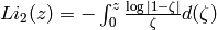
$Li_2(z) = - \int_0^z \frac{\log|1-\zeta|}{\zeta} d(\zeta)$

$= \sum_{k=1}^\infty \frac{z^k}{k}$

Note that the series definition can only be used for $|z| < 1$

EXAMPLES:

sage: a = ComplexNumber(1,0)
sage: a.dilog()
1.64493406684823
sage: float(pi^2/6)
1.6449340668482262

sage: b = ComplexNumber(0,1)
sage: b.dilog()
-0.205616758356028 + 0.915965594177219*I

sage: c = ComplexNumber(0,0)
sage: c.dilog()
0

eta(omit_frac=False)¶

Return the value of the Dedekind $\eta$ function on self, intelligently computed using $\mathbb{SL}(2,\ZZ)$ transformations.

INPUT:

self - element of the upper half plane (if not, raises a ValueError).
omit_frac - (bool, default: False), if True, omit the $e^{\pi i z / 12}$ factor.

OUTPUT: a complex number

The $\eta$ function is

$\eta(z) = e^{\pi i z / 12} \prod_{n=1}^{\infty}(1-e^{2\pi inz})$

ALGORITHM: Uses the PARI C library.

EXAMPLES:

First we compute $\eta(1+i)$ :

sage: i = CC.0
sage: z = 1+i; z.eta()
0.742048775836565 + 0.198831370229911*I

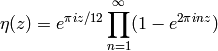
We compute eta to low precision directly from the definition.

sage: z = 1 + i; z.eta()
0.742048775836565 + 0.198831370229911*I
sage: pi = CC(pi)        # otherwise we will get a symbolic result.
sage: exp(pi * i * z / 12) * prod([1-exp(2*pi*i*n*z) for n in range(1,10)])
0.742048775836565 + 0.198831370229911*I

The optional argument allows us to omit the fractional part:

sage: z = 1 + i
sage: z.eta(omit_frac=True)
0.998129069925959 - 8.12769318...e-22*I
sage: prod([1-exp(2*pi*i*n*z) for n in range(1,10)])
0.998129069925958 + 4.59099857829247e-19*I

We illustrate what happens when $z$ is not in the upper half plane.

sage: z = CC(1)
sage: z.eta()
...
ValueError: value must be in the upper half plane

You can also use functional notation.

sage: eta(1+CC(I))
0.742048775836565 + 0.198831370229911*I

exp()¶

Compute exp(z).

EXAMPLES:

sage: i = ComplexField(300).0
sage: z = 1 + i
sage: z.exp()
1.46869393991588515713896759732660426132695673662900872279767567631093696585951213872272450 + 2.28735528717884239120817190670050180895558625666835568093865811410364716018934540926734485*I

gamma()¶

Return the Gamma function evaluated at this complex number.

EXAMPLES:

sage: i = ComplexField(30).0
sage: (1+i).gamma()
0.49801567 - 0.15494983*I

TESTS:

sage: CC(0).gamma()
Infinity

sage: CC(-1).gamma()
Infinity

gamma_inc(t)¶

Return the incomplete Gamma function evaluated at this complex number.

EXAMPLES:

sage: C, i = ComplexField(30).objgen()
sage: (1+i).gamma_inc(2 + 3*i)
0.0020969149 - 0.059981914*I
sage: (1+i).gamma_inc(5)
-0.0013781309 + 0.0065198200*I
sage: C(2).gamma_inc(1 + i)
0.70709210 - 0.42035364*I
sage: CC(2).gamma_inc(5)
0.0404276819945128

imag()¶

Return imaginary part of self.

EXAMPLES:

sage: i = ComplexField(100).0
sage: z = 2 + 3*i
sage: x = z.imag(); x
3.0000000000000000000000000000
sage: x.parent()
Real Field with 100 bits of precision
sage: z.imag_part()
3.0000000000000000000000000000

imag_part()¶

Return imaginary part of self.

EXAMPLES:

sage: i = ComplexField(100).0
sage: z = 2 + 3*i
sage: x = z.imag(); x
3.0000000000000000000000000000
sage: x.parent()
Real Field with 100 bits of precision
sage: z.imag_part()
3.0000000000000000000000000000

is_imaginary()¶

Return True if self is imaginary, i.e. has real part zero.

EXAMPLES:

sage: CC(1.23*i).is_imaginary()
True
sage: CC(1+i).is_imaginary()
False

is_real()¶

Return True if self is real, i.e. has imaginary part zero.

EXAMPLES:

sage: CC(1.23).is_real()
True
sage: CC(1+i).is_real()
False

is_square()¶

This function always returns true as $\CC$ is algebraically closed.

EXAMPLES:

sage: a = ComplexNumber(2,1)
sage: a.is_square()
True

$\CC$ is algebraically closed, hence every element is a square:

sage: b = ComplexNumber(5)
sage: b.is_square()
True

log(base=None)¶

Complex logarithm of z with branch chosen as follows: Write $z = \rho e^{i \theta} with `-\pi < \theta <= pi$ . Then $\mathrm{log}(z) = \mathrm{log}(\rho) + i \theta$ .

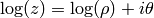Warning

Currently the real log is computed using floats, so there is potential precision loss.

EXAMPLES:

sage: a = ComplexNumber(2,1)
sage: a.log()
0.804718956217050 + 0.463647609000806*I
sage: log(a.abs())
0.804718956217050
sage: a.argument()
0.463647609000806

sage: b = ComplexNumber(float(exp(42)),0)
sage: b.log()
41.99999999999971

sage: c = ComplexNumber(-1,0)
sage: c.log()
3.14159265358979*I

The option of a base is included for compatibility with other logs:

sage: c = ComplexNumber(-1,0)
sage: c.log(2)
4.53236014182719*I

multiplicative_order()¶

Return the multiplicative order of this complex number, if known, or raise a NotImplementedError.

EXAMPLES:

sage: C.<i> = ComplexField()
sage: i.multiplicative_order()
4
sage: C(1).multiplicative_order()
1
sage: C(-1).multiplicative_order()
2
sage: C(i^2).multiplicative_order()
2
sage: C(-i).multiplicative_order()
4
sage: C(2).multiplicative_order()
+Infinity
sage: w = (1+sqrt(-3.0))/2; w
0.500000000000000 + 0.866025403784439*I
sage: abs(w)
1.00000000000000
sage: w.multiplicative_order()
...
NotImplementedError: order of element not known

norm()¶

Returns the norm of this complex number. If $c = a + bi$ is a complex number, then the norm of $c$ is defined as

$\text{norm}(c) = \text{norm}(a + bi) = a^2 + b^2$

The norm of a complex number is different from its absolute value. The absolute value of a complex number is defined to be the square root of its norm. A typical use of the complex norm is in the integral domain $\ZZ[i]$ of Gaussian integers, where the norm of each Gaussian integer $c = a + bi$ is defined as its complex norm.

EXAMPLES:

This indeed acts as the square function when the imaginary component of self is equal to zero:

sage: a = ComplexNumber(2,1)
sage: a.norm()
5.00000000000000
sage: b = ComplexNumber(4.2,0)
sage: b.norm()
17.6400000000000
sage: b^2
17.6400000000000

nth_root(n, all=False)¶

The n-th root function.

INPUT:

all - bool (default: False); if True, return a list of all n-th roots.

EXAMPLES:

sage: a = CC(27)
sage: a.nth_root(3)
3.00000000000000
sage: a.nth_root(3, all=True)
[3.00000000000000, -1.50000000000000 + 2.59807621135332*I, -1.50000000000000 - 2.59807621135332*I]
sage: a = ComplexField(20)(2,1)
sage: [r^7 for r in a.nth_root(7, all=True)]
[2.0000 + 1.0000*I, 2.0000 + 1.0000*I, 2.0000 + 1.0000*I, 2.0000 + 1.0000*I, 2.0000 + 1.0000*I, 2.0000 + 1.0001*I, 2.0000 + 1.0001*I]

plot(**kargs)¶

Plots this complex number as a point in the plane

The accepted options are the ones of point2d(). Type point2d.options to see all options.

Note

Just wraps the sage.plot.point.point2d method

EXAMPLES:

You can either use the indirect:

sage: z = CC(0,1)
sage: plot(z)

or the more direct:

sage: z = CC(0,1)
sage: z.plot()

prec()¶

Return precision of this complex number.

EXAMPLES:

sage: i = ComplexField(2000).0
sage: i.prec()
2000

real()¶

Return real part of self.

EXAMPLES:

sage: i = ComplexField(100).0
sage: z = 2 + 3*i
sage: x = z.real(); x
2.0000000000000000000000000000
sage: x.parent()
Real Field with 100 bits of precision
sage: z.real_part()
2.0000000000000000000000000000

real_part()¶

Return real part of self.

EXAMPLES:

sage: i = ComplexField(100).0
sage: z = 2 + 3*i
sage: x = z.real(); x
2.0000000000000000000000000000
sage: x.parent()
Real Field with 100 bits of precision
sage: z.real_part()
2.0000000000000000000000000000

sec()¶

EXAMPLES:

sage: ComplexField(100)(1,1).sec()
0.49833703055518678521380589177 + 0.59108384172104504805039169297*I

sech()¶

EXAMPLES:

sage: ComplexField(100)(1,1).sech()
0.49833703055518678521380589177 - 0.59108384172104504805039169297*I

sin()¶

EXAMPLES:

sage: (1+CC(I)).sin()
1.29845758141598 + 0.634963914784736*I

sinh()¶

EXAMPLES:

sage: (1+CC(I)).sinh()
0.634963914784736 + 1.29845758141598*I

sqrt(all=False)¶

The square root function, taking the branch cut to be the negative real axis.

INPUT:

all - bool (default: False); if True, return a list of all square roots.

EXAMPLES:

sage: C.<i> = ComplexField(30)
sage: i.sqrt()
0.70710678 + 0.70710678*I
sage: (1+i).sqrt()
1.0986841 + 0.45508986*I
sage: (C(-1)).sqrt()
1.0000000*I
sage: (1 + 1e-100*i).sqrt()^2
1.0000000 + 1.0000000e-100*I
sage: i = ComplexField(200).0
sage: i.sqrt()
0.70710678118654752440084436210484903928483593768847403658834 + 0.70710678118654752440084436210484903928483593768847403658834*I

str(base=10, truncate=True)¶

Return a string representation of this number.

INPUTS:

base - The base to use for printing (default 10)
truncate - (default: True) Whether to print fewer digits than are available, to mask errors in the last bits.

EXAMPLES:

sage: a = CC(pi + I*e)
sage: a.str()
'3.14159265358979 + 2.71828182845905*I'
sage: a.str(truncate=False)
'3.1415926535897931 + 2.7182818284590451*I'
sage: a.str(base=2)
'11.001001000011111101101010100010001000010110100011000 + 10.101101111110000101010001011000101000101011101101001*I'
sage: CC(0.5 + 0.625*I).str(base=2)
'0.10000000000000000000000000000000000000000000000000000 + 0.10100000000000000000000000000000000000000000000000000*I'
sage: a.str(base=16)
'3.243f6a8885a30 + 2.b7e151628aed2*I'
sage: a.str(base=36)
'3.53i5ab8p5fc + 2.puw5nggjf8f*I'

tan()¶

EXAMPLES:

sage: (1+CC(I)).tan()
0.271752585319512 + 1.08392332733869*I

tanh()¶

EXAMPLES:

sage: (1+CC(I)).tanh()
1.08392332733869 + 0.271752585319512*I

zeta()¶

Return the Riemann zeta function evaluated at this complex number.

EXAMPLES:

sage: i = ComplexField(30).gen()
sage: z = 1 + i
sage: z.zeta()
0.58215806 - 0.92684856*I
sage: zeta(z)
0.58215806 - 0.92684856*I

class sage.rings.complex_number.RRtoCC¶: Bases: sage.categories.map.Map

sage.rings.complex_number.cmp_abs(a, b)¶

Returns -1, 0, or 1 according to whether $|a|$ is less than, equal to, or greater than $|b|$ .

Optimized for non-close numbers, where the ordering can be determined by examining exponents.

EXAMPLES:

sage: from sage.rings.complex_number import cmp_abs
sage: cmp_abs(CC(5), CC(1))
1
sage: cmp_abs(CC(5), CC(4))
1
sage: cmp_abs(CC(5), CC(5))
0
sage: cmp_abs(CC(5), CC(6))
-1
sage: cmp_abs(CC(5), CC(100))
-1
sage: cmp_abs(CC(-100), CC(1))
1
sage: cmp_abs(CC(-100), CC(100))
0
sage: cmp_abs(CC(-100), CC(1000))
-1
sage: cmp_abs(CC(1,1), CC(1))
1
sage: cmp_abs(CC(1,1), CC(2))
-1
sage: cmp_abs(CC(1,1), CC(1,0.99999))
1
sage: cmp_abs(CC(1,1), CC(1,-1))
0
sage: cmp_abs(CC(0), CC(1))
-1
sage: cmp_abs(CC(1), CC(0))
1
sage: cmp_abs(CC(0), CC(0))
0
sage: cmp_abs(CC(2,1), CC(1,2))
0

sage.rings.complex_number.create_ComplexNumber(s_real, s_imag=None, pad=0, min_prec=53)¶

Return the complex number defined by the strings s_real and s_imag as an element of ComplexField(prec=n), where n potentially has slightly more (controlled by pad) bits than given by s.

INPUT:

s_real - a string that defines a real number (or something whose string representation defines a number)
s_imag - a string that defines a real number (or something whose string representation defines a number)
pad - an integer >= 0.
min_prec - number will have at least this many bits of precision, no matter what.

EXAMPLES:

sage: ComplexNumber('2.3')
2.30000000000000
sage: ComplexNumber('2.3','1.1')
2.30000000000000 + 1.10000000000000*I
sage: ComplexNumber(10)
10.0000000000000
sage: ComplexNumber(10,10)
10.0000000000000 + 10.0000000000000*I
sage: ComplexNumber(1.000000000000000000000000000,2)
1.00000000000000000000000000 + 2.00000000000000000000000000*I
sage: ComplexNumber(1,2.000000000000000000000)
1.00000000000000000000 + 2.00000000000000000000*I

sage: sage.rings.complex_number.create_ComplexNumber(s_real=2,s_imag=1)
2.00000000000000 + 1.00000000000000*I

sage.rings.complex_number.is_ComplexNumber(x)¶

Returns True if x is a complex number. In particular, if x is of the ComplexNumber type.

EXAMPLES:

sage: from sage.rings.complex_number import is_ComplexNumber
sage: a = ComplexNumber(1,2); a
1.00000000000000 + 2.00000000000000*I
sage: is_ComplexNumber(a)
True
sage: b = ComplexNumber(1); b
1.00000000000000
sage: is_ComplexNumber(b)
True

Note that the global element I is of type SymbolicConstant. However, elements of the class ComplexField_class are of type ComplexNumber:

sage: c = 1 + 2*I
sage: is_ComplexNumber(c)
False
sage: d = CC(1 + 2*I)
sage: is_ComplexNumber(d)
True

sage.rings.complex_number.make_ComplexNumber0(fld, mult_order, re, im)¶

sage.rings.complex_number.set_global_complex_round_mode(n)¶

Arbitrary Precision Complex Numbers¶

Previous topic

Next topic

This Page

Navigation

Arbitrary Precision Complex Numbers¶

Previous topic

Next topic

This Page

Quick search

Navigation