Finite Delta-complexes¶

AUTHORS:

John H. Palmieri (2009-08)

This module implements the basic structure of finite $\Delta$ -complexes. For full mathematical details, see Hatcher [Hat], especially Section 2.1 and the Appendix on “Simplicial CW Structures”. As Hatcher points out, $\Delta$ -complexes were first introduced by Eilenberg and Zilber [EZ], although they called them “semi-simplicial complexes”.

A $\Delta$ -complex is a generalization of a simplicial complex; a $\Delta$ -complex $X$ consists of sets $X_n$ for each non-negative integer $n$ , the elements of which are called n-simplices, along with face maps between these sets of simplices: for each $n$ and for all $0 \leq i \leq n$ , there are functions $d_i$ from $X_n$ to $X_{n-1}$ , with $d_i(s)$ equal to the $i$ -th face of $s$ for each simplex $s \in X_n$ . These maps must satisfy the simplicial identity

$d_i d_j = d_{j-1} d_i \text{ for all } i<j.$

Given a $\Delta$ -complex, it has a geometric realization: a topological space built by taking one topological $n$ -simplex for each element of $X_n$ , and gluing them together as determined by the face maps.

$\Delta$ -complexes are an alternative to simplicial complexes. Every simplicial complex is automatically a $\Delta$ -complex; in the other direction, though, it seems in practice that one can often construct $\Delta$ -complex representations for spaces with many fewer simplices than in a simplicial complex representation. For example, the minimal triangulation of a torus as a simplicial complex contains 14 triangles, 21 edges, and 7 vertices, while there is a $\Delta$ -complex representation of a torus using only 2 triangles, 3 edges, and 1 vertex.

Note

This class derives from GenericCellComplex, and so inherits its methods. Some of those methods are not listed here; see the Generic Cell Complex page instead.

REFERENCES:

[Hat]

Allen Hatcher, “Algebraic Topology”, Cambridge University Press (2002).

[EZ]	S. Eilenberg and J. Zilber, “Semi-Simplicial Complexes and Singular Homology”, Ann. Math. (2) 51 (1950), 499-513.

class sage.homology.delta_complex.DeltaComplex(data=None, **kwds)¶

Bases: sage.homology.cell_complex.GenericCellComplex

Define a $\Delta$ -complex.

Parameters:	data – see below for a description of the options check_validity (boolean; optional, default True) – If True, check that the simplicial identities hold.
Returns:	a $\Delta$ -complex

Use data to define a $\Delta$ -complex. It may be in any of three forms:

data may be a dictionary indexed by simplices. The value associated to a d-simplex $S$ can be any of:
- a list or tuple of (d-1)-simplices, where the ith entry is the ith face of S, given as a simplex,
- another d-simplex $T$ , in which case the ith face of $S$ is declared to be the same as the ith face of $T$ : $S$ and $T$ are glued along their entire boundary,
- None or True or False or anything other than the previous two options, in which case the faces are just the ordinary faces of $S$ .
For example, consider the following:
```
sage: n = 5
sage: S5 = DeltaComplex({Simplex(n):True, Simplex(range(1,n+2)): Simplex(n)})
sage: S5
Delta complex with 6 vertices and 65 simplices
```
The first entry in dictionary forming the argument to DeltaComplex says that there is an $n$ -dimensional simplex with its ordinary boundary. The second entry says that there is another simplex whose boundary is glued to that of the first one. The resulting $\Delta$ -complex is, of course, homeomorphic to an $n$ -sphere, or actually a 5-sphere, since we defined $n$ to be 5. (Note that the second simplex here can be any $n$ -dimensional simplex, as long as it is distinct from Simplex(n).)

Let’s compute its homology, and also compare it to the simplicial version:
```
sage: S5.homology()
{0: 0, 1: 0, 2: 0, 3: 0, 4: 0, 5: Z}
sage: S5.f_vector()  # number of simplices in each dimension
[1, 6, 15, 20, 15, 6, 2]
sage: simplicial_complexes.Sphere(5).f_vector()
[1, 7, 21, 35, 35, 21, 7]
```
Both contain a single (-1)-simplex, the empty simplex; other than that, the $\Delta$ -complex version contains fewer simplices than the simplicial one in each dimension.

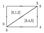
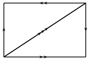
To construct a torus, use:
```
sage: torus_dict = {Simplex([0,1,2]): True,
...          Simplex([3,4,5]): (Simplex([0,1]), Simplex([0,2]), Simplex([1,2])),
...          Simplex([0,1]): (Simplex(0), Simplex(0)),
...          Simplex([0,2]): (Simplex(0), Simplex(0)),
...          Simplex([1,2]): (Simplex(0), Simplex(0)),
...          Simplex(0): ()}
sage: T = DeltaComplex(torus_dict); T
Delta complex with 1 vertex and 7 simplices
sage: T.cohomology(base_ring=QQ)
{0: Vector space of dimension 0 over Rational Field,
 1: Vector space of dimension 2 over Rational Field,
 2: Vector space of dimension 1 over Rational Field}
```
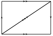
This $\Delta$ -complex consists of two triangles (given by Simplex([0,1,2]) and Simplex([3,4,5])); the boundary of the first is just its usual boundary: the 0th face is obtained by omitting the lowest numbered vertex, etc., and so the boundary consists of the edges [1,2], [0,2], and [0,1], in that order. The boundary of the second is, on the one hand, computed the same way: the nth face is obtained by omitting the nth vertex. On the other hand, the boundary is explicitly declared to be edges [0,1], [0,2], and [1,2], in that order. This glues the second triangle to the first in the prescribed way. The three edges each start and end at the single vertex, Simplex(0).
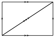
data may be nested lists or tuples. The nth entry in the list is a list of the n-simplices in the complex, and each n-simplex is encoded as a list, the ith entry of which is its ith face. Each face is represented by an integer, giving its index in the list of (n-1)-faces. For example, consider this:
```
sage: P = DeltaComplex( [ [(), ()],  [(1,0), (1,0), (0,0)],
...                       [(1,0,2), (0, 1, 2)] ])
```
The 0th entry in the list is [(), ()]: there are two 0-simplices, and their boundaries are empty.

The 1st entry in the list is [(1,0), (1,0), (0,0)]: there are three 1-simplices. Two of them have boundary (1,0), which means that their 0th face is vertex 1 (in the list of vertices), and their 1st face is vertex 0. The other edge has boundary (0,0), so it starts and ends at vertex 0.

The 2nd entry in the list is [(1,0,2), (0,1,2)]: there are two 2-simplices. The first 2-simplex has boundary (1,0,2), meaning that its 0th face is edge 1 (in the list above), its 1st face is edge 0, and its 2nd face is edge 2; similarly for the 2nd 2-simplex.

If one draws two triangles and identifies them according to this description, the result is the real projective plane.
```
sage: P.homology(1)
C2
sage: P.cohomology(2)
C2
```
Closely related to this form for data is X.cells() for a $\Delta$ -complex X: this is a dictionary, indexed by dimension d, whose d-th entry is a list of the d-simplices, as a list:
```
sage: P.cells()
{0: ((), ()), 1: ((1, 0), (1, 0), (0, 0)), 2: ((1, 0, 2), (0, 1, 2)), -1: ((),)}
```

data may be a dictionary indexed by integers. For each integer $n$ , the entry with key $n$ is the list of $n$ -simplices: this is the same format as is output by the cells() method.

sage: P = DeltaComplex( [ [(), ()],  [(1,0), (1,0), (0,0)],
...                       [(1,0,2), (0, 1, 2)] ])
sage: cells_dict = P.cells()
sage: cells_dict
{0: ((), ()), 1: ((1, 0), (1, 0), (0, 0)), 2: ((1, 0, 2), (0, 1, 2)), -1: ((),)}
sage: DeltaComplex(cells_dict)
Delta complex with 2 vertices and 8 simplices
sage: P == DeltaComplex(cells_dict)
True

Since $\Delta$ -complexes are generalizations of simplicial complexes, any simplicial complex may be viewed as a $\Delta$ -complex:

sage: RP2 = simplicial_complexes.RealProjectivePlane()
sage: RP2_delta = RP2.delta_complex()
sage: RP2.f_vector()
[1, 6, 15, 10]
sage: RP2_delta.f_vector()
[1, 6, 15, 10]

Finally, $\Delta$ -complex constructions for several familiar spaces are available as follows:

sage: delta_complexes.Sphere(4)  # the 4-sphere
Delta complex with 5 vertices and 33 simplices
sage: delta_complexes.KleinBottle()
Delta complex with 1 vertex and 7 simplices
sage: delta_complexes.RealProjectivePlane()
Delta complex with 2 vertices and 8 simplices

Type delta_complexes. and then hit the TAB key to get the full list.

barycentric_subdivision()¶

Not implemented.

EXAMPLES:

sage: K = delta_complexes.KleinBottle()
sage: K.barycentric_subdivision()
...
NotImplementedError: Barycentric subdivisions are not implemented for Delta complexes.

cells(subcomplex=None)¶

The cells of this $\Delta$ -complex.

Parameter:	subcomplex (optional, default None) – a subcomplex of this complex

The cells of this $\Delta$ -complex, in the form of a dictionary: the keys are integers, representing dimension, and the value associated to an integer d is the list of d-cells. Each d-cell is further represented by a list, the ith entry of which gives the index of its ith face in the list of (d-1)-cells.

If the optional argument subcomplex is present, then “return only the faces which are not in the subcomplex”. To preserve the indexing, which is necessary to compute the relative chain complex, this actually replaces the faces in subcomplex with None.

EXAMPLES:

sage: S2 = delta_complexes.Sphere(2)
sage: S2.cells()
{0: ((), (), ()), 1: ((0, 1), (0, 2), (1, 2)), 2: ((0, 1, 2), (0, 1, 2)), -1: ((),)}
sage: A = S2.subcomplex({1: [0,2]}) # one edge
sage: S2.cells(subcomplex=A)
{0: (None, None, None), 1: (None, (0, 2), None), 2: ((0, 1, 2), (0, 1, 2)), -1: (None,)}

chain_complex(**kwds)¶

The chain complex associated to this $\Delta$ -complex.

Parameters:

dimensions – if None, compute the chain complex in all dimensions. If a list or tuple of integers, compute the chain complex in those dimensions, setting the chain groups in all other dimensions to zero. NOT IMPLEMENTED YET: this function always returns the entire chain complex
base_ring (optional, default ZZ) – commutative ring
subcomplex (optional, default empty) – a subcomplex of this simplicial complex. Compute the chain complex relative to this subcomplex.
augmented (boolean; optional, default False) – If True, return the augmented chain complex (that is, include a class in dimension $-1$ corresponding to the empty cell). This is ignored if dimensions is specified or if subcomplex is nonempty.
cochain (boolean; optional, default False) – If True, return the cochain complex (that is, the dual of the chain complex).
verbose (boolean; optional, default False) – If True, print some messages as the chain complex is computed.
check_diffs (boolean; optional, default False) – If True, make sure that the chain complex is actually a chain complex: the differentials are composable and their product is zero.

Note

If subcomplex is nonempty, then the argument augmented has no effect: the chain complex relative to a nonempty subcomplex is zero in dimension $-1$ .

EXAMPLES:

sage: circle = delta_complexes.Sphere(1)
sage: circle.chain_complex()
Chain complex with at most 2 nonzero terms over Integer Ring
sage: circle.chain_complex()._latex_()
'\\Bold{Z}^{1} \\xrightarrow{d_{1}} \\Bold{Z}^{1}'
sage: circle.chain_complex(base_ring=QQ, augmented=True)
Chain complex with at most 3 nonzero terms over Rational Field
sage: circle.homology(dim=1)
Z
sage: circle.cohomology(dim=1)
Z
sage: T = T = delta_complexes.Torus()
sage: T.chain_complex(subcomplex=T)
Chain complex with at most 0 nonzero terms over Integer Ring
sage: T.homology(subcomplex=T)
{0: 0, 1: 0, 2: 0}
sage: A = T.subcomplex({2: [1]})  # one of the two triangles forming T
sage: T.chain_complex(subcomplex=A)
Chain complex with at most 1 nonzero terms over Integer Ring
sage: T.homology(subcomplex=A)
{0: 0, 1: 0, 2: Z}

cone()¶

The cone on this $\Delta$ -complex.

The cone is the complex formed by adding a new vertex $C$ and simplices of the form $[C, v_0, ..., v_k]$ for every simplex $[v_0, ..., v_k]$ in the original complex. That is, the cone is the join of the original complex with a one-point complex.

EXAMPLES:

sage: K = delta_complexes.KleinBottle()
sage: K.cone()
Delta complex with 2 vertices and 14 simplices
sage: K.cone().homology()
{0: 0, 1: 0, 2: 0, 3: 0}

connected_sum(other)¶

Return the connected sum of self with other.

Parameter:	other – another $\Delta$ -complex
Returns:	the connected sum `self # other`

Warning

This does not check that self and other are manifolds. It doesn’t even check that their facets all have the same dimension. It just chooses top-dimensional simplices from each complex, checks that they have the same dimension, removes them, and glues the remaining pieces together. Since a (more or less) random facet is chosen from each complex, this method may return random results if applied to non-manifolds, depending on which facet is chosen.

ALGORITHM:

Pick a top-dimensional simplex from each complex. Check to see if there are any identifications on either simplex, using the _is_glued() method. If there are no identifications, remove the simplices and glue the remaining parts of complexes along their boundary. If there are identifications on a simplex, subdivide it repeatedly (using elementary_subdivision()) until some piece has no identifications.

EXAMPLES:

sage: T = delta_complexes.Torus()
sage: S2 = delta_complexes.Sphere(2)
sage: T.connected_sum(S2).cohomology() == T.cohomology()
True
sage: RP2 = delta_complexes.RealProjectivePlane()
sage: T.connected_sum(RP2).homology(1)
Z x Z x C2
sage: T.connected_sum(RP2).homology(2)
0
sage: RP2.connected_sum(RP2).connected_sum(RP2).homology(1)
Z x Z x C2

disjoint_union(right)¶

The disjoint union of this $\Delta$ -complex with another one.

Parameter:	right – the other $\Delta$ -complex (the right-hand factor)

EXAMPLES:

sage: S1 = delta_complexes.Sphere(1)
sage: S2 = delta_complexes.Sphere(2)
sage: S1.disjoint_union(S2).homology()
{0: Z, 1: Z, 2: Z}

elementary_subdivision(idx=-1)¶

Perform an “elementary subdivision” on a top-dimensional simplex in this $\Delta$ -complex. If the optional argument idx is present, it specifies the index (in the list of top-dimensional simplices) of the simplex to subdivide. If not present, subdivide the last entry in this list.

Parameter:	idx (integer; optional, default -1) – index specifying which simplex to subdivide
Returns:	$\Delta$ -complex with one simplex subdivided.

Elementary subdivision of a simplex means replacing that simplex with the cone on its boundary. That is, given a $\Delta$ -complex containing an $d$ -simplex $S$ with vertices $v_0$ , ..., $v_d$ , form a new $\Delta$ -complex by

removing $S$
adding a vertex $w$ (thought of as being in the interior of $S$ )
adding all simplices with vertices $v_{i_0}$ , ..., $v_{i_k}$ , $w$ , preserving any identifications present along the boundary of $S$

The algorithm for achieving this uses _epi_from_standard_simplex() to keep track of simplices (with multiplicity) and what their faces are: this method defines a surjection $\pi$ from the standard $d$ -simplex to $S$ . So first remove $S$ and add a new vertex $w$ , say at the end of the old list of vertices. Then for each vertex $v$ in the standard $d$ -simplex, add an edge from $\pi(v)$ to $w$ ; for each edge $(v_0, v_1)$ in the standard $d$ -simplex, add a triangle $(\pi(v_0), \pi(v_1), w)$ , etc.

Note that given an $n$ -simplex $(v_0, v_1, ..., v_n)$ in the standard $d$ -simplex, the faces of the new $(n+1)$ -simplex are given by removing vertices, one at a time, from $(\pi(v_0), ..., \pi(v_n), w)$ . These are either the image of the old $n$ -simplex (if $w$ is removed) or the various new $n$ -simplices added in the previous dimension. So keep track of what’s added in dimension $n$ for use in computing the faces in dimension $n+1$ .

In contrast with barycentric subdivision, note that only the interior of $S$ has been changed; this allows for subdivision of a single top-dimensional simplex without subdividing every simplex in the complex.

The term “elementary subdivison” is taken from p. 112 in John M. Lee’s book [Lee].

REFERENCES:

[Lee]

John M. Lee, Introduction to Topological Manifolds, Springer-Verlag, GTM volume 202.

EXAMPLES:

sage: T = delta_complexes.Torus()
sage: T.n_cells(2)
[(1, 2, 0), (0, 2, 1)]
sage: T.elementary_subdivision(0)  # subdivide first triangle
Delta complex with 2 vertices and 13 simplices
sage: X = T.elementary_subdivision(); X  # subdivide last triangle
Delta complex with 2 vertices and 13 simplices
sage: X.elementary_subdivision()
Delta complex with 3 vertices and 19 simplices
sage: X.homology() == T.homology()
True

face_poset()¶

The face poset of this $\Delta$ -complex, the poset of nonempty cells, ordered by inclusion.

EXAMPLES:

sage: T = delta_complexes.Torus()
sage: T.face_poset()
Finite poset containing 6 elements

graph()¶

The 1-skeleton of this $\Delta$ -complex as a graph.

EXAMPLES:

sage: T = delta_complexes.Torus()
sage: T.graph()
Looped multi-graph on 1 vertex
sage: S = delta_complexes.Sphere(2)
sage: S.graph()
Graph on 3 vertices
sage: delta_complexes.Simplex(4).graph() == graphs.CompleteGraph(5)
True

join(other)¶

The join of this $\Delta$ -complex with another one.

Parameter:	other – another $\Delta$ -complex (the right-hand factor)
Returns:	the join `self * other`

The join of two $\Delta$ -complexes $S$ and $T$ is the $\Delta$ -complex $S*T$ with simplices of the form $[v_0, ..., v_k, w_0, ..., w_n]$ for all simplices $[v_0, ..., v_k]$ in $S$ and $[w_0, ..., w_n]$ in $T$ . The faces are computed accordingly: the ith face of such a simplex is either $(d_i S) * T$ if $i \leq k$ , or $S * (d_{i-k-1} T)$ if $i > k$ .

EXAMPLES:

sage: T = delta_complexes.Torus()
sage: S0 = delta_complexes.Sphere(0)
sage: T.join(S0)  # the suspension of T
Delta complex with 3 vertices and 21 simplices

Compare to simplicial complexes:

sage: K = delta_complexes.KleinBottle()
sage: T_simp = simplicial_complexes.Torus()
sage: K_simp = simplicial_complexes.KleinBottle()
sage: T.join(K).homology()[3] == T_simp.join(K_simp).homology()[3] # long time (3 seconds)
True

The notation ‘*’ may be used, as well:

sage: S1 = delta_complexes.Sphere(1)
sage: X = S1 * S1    # X is a 3-sphere
sage: X.homology()
{0: 0, 1: 0, 2: 0, 3: Z}

n_skeleton(n)¶

The n-skeleton of this $\Delta$ -complex.

Parameter:	n (non-negative integer) – dimension

EXAMPLES:

sage: S3 = delta_complexes.Sphere(3)
sage: S3.n_skeleton(1) # 1-skeleton of a tetrahedron
Delta complex with 4 vertices and 11 simplices
sage: S3.n_skeleton(1).dimension()
1
sage: S3.n_skeleton(1).homology()
{0: 0, 1: Z x Z x Z}

product(other)¶

The product of this $\Delta$ -complex with another one.

Parameter:	other – another $\Delta$ -complex (the right-hand factor)
Returns:	the product `self x other`

Warning

If X and Y are $\Delta$ -complexes, then X*Y returns their join, not their product.

EXAMPLES:

sage: K = delta_complexes.KleinBottle()
sage: X = K.product(K)
sage: X.homology(1)
Z x Z x C2 x C2
sage: X.homology(2)
Z x C2 x C2 x C2
sage: X.homology(3)
C2
sage: X.homology(4)
0
sage: X.homology(base_ring=GF(2))
{0: Vector space of dimension 0 over Finite Field of size 2,
 1: Vector space of dimension 4 over Finite Field of size 2,
 2: Vector space of dimension 6 over Finite Field of size 2,
 3: Vector space of dimension 4 over Finite Field of size 2,
 4: Vector space of dimension 1 over Finite Field of size 2}
sage: S1 = delta_complexes.Sphere(1)
sage: K.product(S1).homology() == S1.product(K).homology()
True
sage: S1.product(S1) == delta_complexes.Torus()
True

subcomplex(data)¶

Create a subcomplex.

Parameter:	data – a dictionary indexed by dimension or a list (or tuple); in either case, data[n] should be the list (or tuple or set) of the indices of the simplices to be included in the subcomplex.

This automatically includes all faces of the simplices in data, so you only have to specify the simplices which are maximal with respect to inclusion.

EXAMPLES:

sage: X = delta_complexes.Torus()
sage: A = X.subcomplex({2: [0]})  # one of the triangles of X
sage: X.homology(subcomplex=A)
{0: 0, 1: 0, 2: Z}

In the following, line is a line segment and ends is the complex consisting of its two endpoints, so the relative homology of the two is isomorphic to the homology of a circle:

sage: line = delta_complexes.Simplex(1) # an edge
sage: line.cells()
{0: ((), ()), 1: ((0, 1),), -1: ((),)}
sage: ends = line.subcomplex({0: (0, 1)})
sage: ends.cells()
{0: ((), ()), -1: ((),)}
sage: line.homology(subcomplex=ends)
{0: 0, 1: Z}

suspension(n=1)¶

The suspension of this $\Delta$ -complex.

Parameter:	n (positive integer; optional, default 1) – suspend this many times.

The suspension is the complex formed by adding two new vertices $S_0$ and $S_1$ and simplices of the form $[S_0, v_0, ..., v_k]$ and $[S_1, v_0, ..., v_k]$ for every simplex $[v_0, ..., v_k]$ in the original complex. That is, the suspension is the join of the original complex with a two-point complex (the 0-sphere).

EXAMPLES:

sage: S = delta_complexes.Sphere(0)
sage: S3 = S.suspension(3)  # the 3-sphere
sage: S3.homology()
{0: 0, 1: 0, 2: 0, 3: Z}

wedge(right)¶

The wedge (one-point union) of this $\Delta$ -complex with another one.

Parameter:	right – the other $\Delta$ -complex (the right-hand factor)

Note

This operation is not well-defined if self or other is not path-connected.

EXAMPLES:

sage: S1 = delta_complexes.Sphere(1)
sage: S2 = delta_complexes.Sphere(2)
sage: S1.wedge(S2).homology()
{0: 0, 1: Z, 2: Z}

class sage.homology.delta_complex.DeltaComplexExamples¶

Some examples of $\Delta$ -complexes.

Here are the available examples; you can also type delta_complexes. and hit TAB to get a list:

Sphere
Torus
RealProjectivePlane
KleinBottle
Simplex
SurfaceOfGenus

EXAMPLES:

sage: S = delta_complexes.Sphere(6) # the 6-sphere
sage: S.dimension()
6
sage: S.cohomology(6)
Z
sage: delta_complexes.Torus() == delta_complexes.Sphere(3)
False

KleinBottle()¶

A $\Delta$ -complex representation of the Klein bottle, consisting of one vertex, three edges, and two triangles.

EXAMPLES:

sage: delta_complexes.KleinBottle()
Delta complex with 1 vertex and 7 simplices

RealProjectivePlane()¶

A $\Delta$ -complex representation of the real projective plane, consisting of two vertices, three edges, and two triangles.

EXAMPLES:

sage: P = delta_complexes.RealProjectivePlane()
sage: P.cohomology(1)
0
sage: P.cohomology(2)
C2
sage: P.cohomology(dim=1, base_ring=GF(2))
Vector space of dimension 1 over Finite Field of size 2
sage: P.cohomology(dim=2, base_ring=GF(2))
Vector space of dimension 1 over Finite Field of size 2

Simplex(n)¶

A $\Delta$ -complex representation of an $n$ -simplex, consisting of a single $n$ -simplex and its faces. (This is the same as the simplicial complex representation available by using simplicial_complexes.Simplex(n).)

EXAMPLES:

sage: delta_complexes.Simplex(3)
Delta complex with 4 vertices and 16 simplices

Sphere(n)¶

A $\Delta$ -complex representation of the $n$ -dimensional sphere, formed by gluing two $n$ -simplices along their boundary, except in dimension 1, in which case it is a single 1-simplex starting and ending at the same vertex.

Parameter:	n – dimension of the sphere

EXAMPLES:

sage: delta_complexes.Sphere(4).cohomology(4, base_ring=GF(3))
Vector space of dimension 1 over Finite Field of size 3

SurfaceOfGenus(g, orientable=True)¶

A surface of genus g as a $\Delta$ -complex.

Parameters:	g (non-negative integer) – the genus orientable (bool, optional, default True) – whether the surface should be orientable

In the orientable case, return a sphere if $g$ is zero, and otherwise return a $g$ -fold connected sum of a torus with itself.

In the non-orientable case, raise an error if $g$ is zero. If $g$ is positive, return a $g$ -fold connected sum of a real projective plane with itself.

EXAMPLES:

sage: delta_complexes.SurfaceOfGenus(1, orientable=False)
Delta complex with 2 vertices and 8 simplices
sage: delta_complexes.SurfaceOfGenus(3, orientable=False).homology(1)
Z x Z x C2
sage: delta_complexes.SurfaceOfGenus(3, orientable=False).homology(2)
0

Compare to simplicial complexes:

sage: delta_g4 = delta_complexes.SurfaceOfGenus(4)
sage: delta_g4.f_vector()
[1, 5, 33, 22]
sage: simpl_g4 = simplicial_complexes.SurfaceOfGenus(4)
sage: simpl_g4.f_vector()
[1, 19, 75, 50]
sage: delta_g4.homology() == simpl_g4.homology()
True            

Torus()¶

A $\Delta$ -complex representation of the torus, consisting of one vertex, three edges, and two triangles.

EXAMPLES:

sage: delta_complexes.Torus().homology(1)
Z x Z

Finite Delta-complexes¶

Previous topic

Next topic

This Page

Navigation

Finite Delta-complexes¶

Previous topic

Next topic

This Page

Quick search

Navigation