Finite simplicial complexes¶

AUTHORS:

John H. Palmieri (2009-04)
D. Benjamin Antieau (2009-06) - added is_connected, generated_subcomplex, remove_facet, and is_flag_complex methods; cached the output of the graph() method.

This module implements the basic structure of finite simplicial complexes. Given a set $V$ of “vertices”, a simplicial complex on $V$ is a collection $K$ of subsets of $V$ satisfying the condition that if $S$ is one of the subsets in $K$ , then so is every subset of $S$ . The subsets $S$ are called the ‘simplices’ of $K$ .

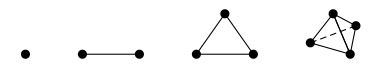
A simplicial complex $K$ can be viewed as a purely combinatorial object, as described above, but it also gives rise to a topological space $|K|$ (its geometric realization) as follows: first, the points of $V$ should be in general position in euclidean space. Next, if $\{v\}$ is in $K$ , then the vertex $v$ is in $|K|$ . If $\{v, w\}$ is in $K$ , then the line segment from $v$ to $w$ is in $|K|$ . If $\{u, v, w\}$ is in $K$ , then the triangle with vertices $u$ , $v$ , and $w$ is in $|K|$ . In general, $|K|$ is the union of the convex hulls of simplices of $K$ . Frequently, one abuses notation and uses $K$ to denote both the simplicial complex and the associated topological space.

For any simplicial complex $K$ and any commutative ring $R$ there is an associated chain complex, with differential of degree $-1$ . The $n^{th}$ term is the free $R$ -module with basis given by the $n$ -simplices of $K$ . The differential is determined by its value on any simplex: on the $n$ -simplex with vertices $(v_0, v_1, ..., v_n)$ , the differential is the alternating sum with $i^{th}$ summand $(-1)^i$ multiplied by the $(n-1)$ -simplex obtained by omitting vertex $v_i$ .

In the implementation here, the vertex set must be finite. To define a simplicial complex, specify its vertex set: this should be a list, tuple, or set, or it can be a non-negative integer $n$ , in which case the vertex set is $(0, ..., n)$ . Also specify the facets: the maximal faces.

Note

The elements of the vertex set are not automatically contained in the simplicial complex: each one is only included if and only if it is a vertex of at least one of the specified facets.

Note

This class derives from GenericCellComplex, and so inherits its methods. Some of those methods are not listed here; see the Generic Cell Complex page instead.

EXAMPLES:

sage: SimplicialComplex([1, 3, 7], [[1], [3, 7]])
Simplicial complex with vertex set (1, 3, 7) and facets {(3, 7), (1,)}
sage: SimplicialComplex(2)   # the empty simplicial complex
Simplicial complex with vertex set (0, 1, 2) and facets {()}
sage: X = SimplicialComplex(3, [[0,1], [1,2], [2,3], [3,0]])
sage: X
Simplicial complex with vertex set (0, 1, 2, 3) and facets {(1, 2), (2, 3), (0, 3), (0, 1)}    
sage: X.stanley_reisner_ring()
Quotient of Multivariate Polynomial Ring in x0, x1, x2, x3 over Integer Ring by the ideal (x1*x3, x0*x2)
sage: X.is_pure()
True

Sage can perform a number of operations on simplicial complexes, such as the join and the product, and it can also compute homology:

sage: S = SimplicialComplex(2, [[0,1], [1,2], [0,2]]) # circle
sage: T = S.product(S)  # torus
sage: T
Simplicial complex with 9 vertices and 18 facets
sage: T.homology()   # this computes reduced homology
{0: 0, 1: Z x Z, 2: Z}
sage: T.euler_characteristic()
0

Sage knows about some basic combinatorial data associated to a simplicial complex:

sage: X = SimplicialComplex(3, [[0,1], [1,2], [2,3], [0,3]])
sage: X.f_vector()
[1, 4, 4]
sage: X.face_poset()
Finite poset containing 8 elements
sage: X.stanley_reisner_ring()
Quotient of Multivariate Polynomial Ring in x0, x1, x2, x3 over Integer Ring by the ideal (x1*x3, x0*x2)

class sage.homology.simplicial_complex.Simplex(X)¶

Bases: sage.structure.sage_object.SageObject

Define a simplex.

Topologically, a simplex is the convex hull of a collection of vertices in general position. Combinatorially, it is defined just by specifying a set of vertices. It is represented in Sage by the tuple of the vertices.

Parameter:	X (integer or list, tuple, or other iterable) – set of vertices
Returns:	simplex with those vertices

X may be a non-negative integer $n$ , in which case the simplicial complex will have $n+1$ vertices $(0, 1, ..., n)$ , or it may be anything which may be converted to a tuple, in which case the vertices will be that tuple. In the second case, each vertex must be hashable, so it should be a number, a string, or a tuple, for instance, but not a list.

Warning

The vertices should be distinct, and no error checking is done to make sure this is the case.

EXAMPLES:

sage: Simplex(4)
(0, 1, 2, 3, 4)
sage: Simplex([3, 4, 1])
(3, 4, 1)
sage: X = Simplex((3, 'a', 'vertex')); X
(3, 'a', 'vertex')
sage: X == loads(dumps(X))
True

Vertices may be tuples but not lists:

sage: Simplex([(1,2), (3,4)])
((1, 2), (3, 4))
sage: Simplex([[1,2], [3,4]])
...
TypeError: unhashable type: 'list'

dimension()¶

The dimension of this simplex: the number of vertices minus 1.

EXAMPLES:

sage: Simplex(5).dimension() == 5
True
sage: Simplex(5).face(1).dimension()
4

face(n)¶

The nth face of this simplex.

Parameter:	n (integer) – an integer between 0 and the dimension of this simplex
Returns:	the simplex obtained by removing the nth vertex from this simplex

EXAMPLES:

sage: S = Simplex(4)
sage: S.face(0)
(1, 2, 3, 4)
sage: S.face(3)
(0, 1, 2, 4)

faces()¶

The list of faces (of codimension 1) of this simplex.

EXAMPLES:

sage: S = Simplex(4)
sage: S.faces()
[(1, 2, 3, 4), (0, 2, 3, 4), (0, 1, 3, 4), (0, 1, 2, 4), (0, 1, 2, 3)]
sage: len(Simplex(10).faces())
11

is_empty()¶

Return True iff this simplex is the empty simplex.

EXAMPLES:

sage: [Simplex(n).is_empty() for n in range(-1,4)]
[True, False, False, False, False]

is_face(other)¶

Return True iff this simplex is a face of other.

EXAMPLES:

sage: Simplex(3).is_face(Simplex(5))
True
sage: Simplex(5).is_face(Simplex(2))
False
sage: Simplex(['a', 'b', 'c']).is_face(Simplex(8))
False

join(right, rename_vertices=True)¶

The join of this simplex with another one.

The join of two simplices $[v_0, ..., v_k]$ and $[w_0, ..., w_n]$ is the simplex $[v_0, ..., v_k, w_0, ..., w_n]$ .

Parameters:

right – the other simplex (the right-hand factor)
rename_vertices (boolean; optional, default True) – If this is True, the vertices in the join will be renamed by this formula: vertex “v” in the left-hand factor –> vertex “Lv” in the join, vertex “w” in the right-hand factor –> vertex “Rw” in the join. If this is false, this tries to construct the join without renaming the vertices; this may cause problems if the two factors have any vertices with names in common.

EXAMPLES:

sage: Simplex(2).join(Simplex(3))
('L0', 'L1', 'L2', 'R0', 'R1', 'R2', 'R3')
sage: Simplex(['a', 'b']).join(Simplex(['x', 'y', 'z']))
('La', 'Lb', 'Rx', 'Ry', 'Rz')
sage: Simplex(['a', 'b']).join(Simplex(['x', 'y', 'z']), rename_vertices=False)
('a', 'b', 'x', 'y', 'z')

product(other, rename_vertices=True)¶

The product of this simplex with another one, as a list of simplices.

Parameters:

other – the other simplex
rename_vertices – If this is False, then the vertices in the product are the set of ordered pairs $(v,w)$ where $v$ is a vertex in the left-hand factor (self) and $w$ is a vertex in the right-hand factor (other). If this is True, then the vertices are renamed as “LvRw” (e.g., the vertex (1,2) would become “L1R2”). This is useful if you want to define the Stanley-Reisner ring of the complex: vertex names like (0,1) are not suitable for that, while vertex names like “L0R1” are.

Algorithm: see Hatcher, p. 277-278 (who in turn refers to Eilenberg-Steenrod, p. 68): given Simplex(m) and Simplex(n), then Simplex(m) x Simplex(n) can be triangulated as follows: for each path $f$ from $(0,0)$ to $(m,n)$ along the integer grid in the plane, going up or right at each lattice point, associate an $(m+n)$ -simplex with vertices $v_0$ , $v_1$ , ..., where $v_k$ is the $k^{th}$ vertex in the path $f$ .

Note that there are $m+n$ choose $n$ such paths. Note also that each vertex in the product is a pair of vertices $(v,w)$ where $v$ is a vertex in the left-hand factor and $w$ is a vertex in the right-hand factor.

Note

This produces a list of simplices – not a Simplex, not a SimplicialComplex.

EXAMPLES:

sage: len(Simplex(2).product(Simplex(2)))
6
sage: Simplex(1).product(Simplex(1))
[('L0R0', 'L0R1', 'L1R1'), ('L0R0', 'L1R0', 'L1R1')]
sage: Simplex(1).product(Simplex(1), rename_vertices=False)
[((0, 0), (0, 1), (1, 1)), ((0, 0), (1, 0), (1, 1))]

REFERENCES:

A. Hatcher, “Algebraic Topology”, Cambridge University Press (2002).

set()¶

The frozenset attached to this simplex.

EXAMPLES:

sage: Simplex(3).set()
frozenset([0, 1, 2, 3])

tuple()¶

The tuple attached to this simplex.

EXAMPLES:

sage: Simplex(3).tuple()
(0, 1, 2, 3)

Although simplices are printed as if they were tuples, they are not the same type:

sage: type(Simplex(3).tuple())
<type 'tuple'>
sage: type(Simplex(3))
<class 'sage.homology.simplicial_complex.Simplex'>

class sage.homology.simplicial_complex.SimplicialComplex(vertex_set=[], maximal_faces=[], **kwds)¶

Bases: sage.homology.cell_complex.GenericCellComplex

Define a simplicial complex.

Parameters:	vertex_set – set of vertices maximal_faces – set of maximal faces vertex_check (boolean; optional, default True) – see below maximality_check (boolean; optional, default True) – see below sort_facets (boolean; optional, default True) – see below name_check (boolean; optional, default False) – see below
Returns:	a simplicial complex

vertex_set may be a non-negative integer $n$ (in which case the simplicial complex will have $n+1$ vertices $\{0, 1, ..., n\}$ ), or it may be anything which may be converted to a tuple. Call the elements of this ‘vertices’.

maximal_faces should be a list or tuple or set (indeed, anything which may be converted to a set) whose elements are lists (or tuples, etc.) of vertices. Maximal faces are also known as ‘facets’.

If vertex_check is True, check to see that each given maximal face is a subset of the vertex set. Raise an error for any bad face.

If maximality_check is True, check that each maximal face is, in fact, maximal. In this case, when producing the internal representation of the simplicial complex, omit those that are not. It is highly recommended that this be True; various methods for this class may fail if faces which are claimed to be maximal are in fact not.

If sort_facets is True, sort the vertices in each facet. If the vertices in different facets are not ordered compatibly (e.g., if you have facets (1, 3, 5) and (5, 3, 8)), then homology calculations may have unpredictable results.

If name_check is True, check the names of the vertices to see if they can be easily converted to generators of a polynomial ring – use this if you plan to use the Stanley-Reisner ring for the simplicial complex.

Note

The elements of vertex_set are not automatically in the simplicial complex: each one is only included if it is a vertex of at least one of the specified facets.

EXAMPLES:

sage: SimplicialComplex(4, [[1,2], [1,4]])
Simplicial complex with vertex set (0, 1, 2, 3, 4) and facets {(1, 2), (1, 4)}
sage: SimplicialComplex(3, [[0,2], [0,3], [0]])
Simplicial complex with vertex set (0, 1, 2, 3) and facets {(0, 2), (0, 3)}
sage: SimplicialComplex(3, [[0,2], [0,3], [0]], maximality_check=False)
Simplicial complex with vertex set (0, 1, 2, 3) and facets {(0, 2), (0, 3), (0,)}
sage: S = SimplicialComplex(['a', 'b', 'c'], (('a', 'b'), ('a', 'c'), ('b', 'c')))
sage: S
Simplicial complex with vertex set ('a', 'b', 'c') and facets {('b', 'c'), ('a', 'c'), ('a', 'b')}

You can also omit the vertex_set argument – if the first argument is a list of lists (or anything similar – something which looks like it should be maximal_faces), then it is used for maximal_faces, and the set of vertices is deduced from the vertices used therein:

sage: SimplicialComplex([[0,2], [0,3], [0,6]])
Simplicial complex with vertex set (0, 2, 3, 6) and facets {(0, 6), (0, 2), (0, 3)}

TESTS:

sage: S = SimplicialComplex(['a', 'b', 'c'], (('a', 'b'), ('a', 'c'), ('b', 'c')))
sage: S == loads(dumps(S))
True

add_face(face)¶

Add a face to this simplicial complex

Parameter:	face – a subset of the vertex set

This changes the simplicial complex, adding a new face and all of its subfaces.

EXAMPLES:

sage: X = SimplicialComplex(2, [[0,1], [0,2]])
sage: X.add_face([0,1,2,]); X
Simplicial complex with vertex set (0, 1, 2) and facets {(0, 1, 2)}
sage: Y = SimplicialComplex(3); Y
Simplicial complex with vertex set (0, 1, 2, 3) and facets {()}
sage: Y.add_face([0,1])
sage: Y.add_face([1,2,3])
sage: Y
Simplicial complex with vertex set (0, 1, 2, 3) and facets {(1, 2, 3), (0, 1)}

If you add a face which is already present, there is no effect:

sage: Y.add_face([1,3]); Y
Simplicial complex with vertex set (0, 1, 2, 3) and facets {(1, 2, 3), (0, 1)}

alexander_dual()¶

The Alexander dual of this simplicial complex: according to the Macaulay2 documentation, this is the simplicial complex whose faces are the complements of its nonfaces.

Thus find the minimal nonfaces and take their complements to find the facets in the Alexander dual.

EXAMPLES:

sage: Y = SimplicialComplex(4); Y
Simplicial complex with vertex set (0, 1, 2, 3, 4) and facets {()}
sage: Y.alexander_dual()
Simplicial complex with vertex set (0, 1, 2, 3, 4) and 5 facets
sage: X = SimplicialComplex(3, [[0,1], [1,2], [2,3], [3,0]])
sage: X.alexander_dual()
Simplicial complex with vertex set (0, 1, 2, 3) and facets {(1, 3), (0, 2)}

barycentric_subdivision()¶

The barycentric subdivision of this simplicial complex.

See http://en.wikipedia.org/wiki/Barycentric_subdivision for a definition.

EXAMPLES:

sage: triangle = SimplicialComplex(2, [[0,1], [1,2], [0, 2]])
sage: hexagon = triangle.barycentric_subdivision()
sage: hexagon
Simplicial complex with 6 vertices and 6 facets
sage: hexagon.homology(1) == triangle.homology(1)
True

Barycentric subdivisions can get quite large, since each $n$ -dimensional facet in the original complex produces $(n+1)!$ facets in the subdivision:

sage: S4 = simplicial_complexes.Sphere(4)
sage: S4
Simplicial complex with vertex set (0, 1, 2, 3, 4, 5) and 6 facets
sage: S4.barycentric_subdivision()
Simplicial complex with 62 vertices and 720 facets

category()¶

Return the category to which this chain complex belongs: the category of all simplicial complexes.

EXAMPLES:

sage: SimplicialComplex(5, [[0,1], [1,2,3,4,5]]).category()
Category of simplicial complexes

cells(subcomplex=None)¶

The faces of this simplicial complex, in the form of a dictionary of sets keyed by dimension. If the optional argument subcomplex is present, then return only the faces which are not in the subcomplex.

Parameter:	subcomplex (optional, default None) – a subcomplex of this simplicial complex. Return faces which are not in this subcomplex.

EXAMPLES:

sage: Y = SimplicialComplex(5, [[1,2], [1,4]])
sage: Y.faces()
{0: set([(4,), (2,), (1,)]), 1: set([(1, 2), (1, 4)]), -1: set([()])}
sage: L = SimplicialComplex(5, [[1,2]])
sage: Y.faces(subcomplex=L)
{0: set([(4,)]), 1: set([(1, 4)]), -1: set([])}

chain_complex(**kwds)¶

The chain complex associated to this simplicial complex.

Parameters:

dimensions – if None, compute the chain complex in all dimensions. If a list or tuple of integers, compute the chain complex in those dimensions, setting the chain groups in all other dimensions to zero.
base_ring (optional, default ZZ) – commutative ring
subcomplex (optional, default empty) – a subcomplex of this simplicial complex. Compute the chain complex relative to this subcomplex.
augmented (boolean; optional, default False) – If True, return the augmented chain complex (that is, include a class in dimension $-1$ corresponding to the empty cell). This is ignored if dimensions is specified.
cochain (boolean; optional, default False) – If True, return the cochain complex (that is, the dual of the chain complex).
verbose (boolean; optional, default False) – If True, print some messages as the chain complex is computed.
check_diffs (boolean; optional, default False) – If True, make sure that the chain complex is actually a chain complex: the differentials are composable and their product is zero.

Note

If subcomplex is nonempty, then the argument augmented has no effect: the chain complex relative to a nonempty subcomplex is zero in dimension $-1$ .

EXAMPLES:

sage: circle = SimplicialComplex(2, [[0,1], [1,2], [0, 2]])
sage: circle.chain_complex()
Chain complex with at most 2 nonzero terms over Integer Ring
sage: circle.chain_complex()._latex_()
'\Bold{Z}^{3} \xrightarrow{d_{1}} \Bold{Z}^{3}'
sage: circle.chain_complex(base_ring=QQ, augmented=True)
Chain complex with at most 3 nonzero terms over Rational Field

cone()¶

The cone on this simplicial complex.

The cone is the simplicial complex formed by adding a new vertex $C$ and simplices of the form $[C, v_0, ..., v_k]$ for every simplex $[v_0, ..., v_k]$ in the original simplicial complex. That is, the cone is the join of the original complex with a one-point simplicial complex.

EXAMPLES:

sage: S = SimplicialComplex(1, [[0], [1]])
sage: S.cone()
Simplicial complex with vertex set ('L0', 'L1', 'R0') and facets {('L0', 'R0'), ('L1', 'R0')}

connected_sum(other)¶

The connected sum of this simplicial complex with another one.

Parameter:	other – another simplicial complex
Returns:	the connected sum `self # other`

Warning

This does not check that self and other are manifolds, only that their facets all have the same dimension. Since a (more or less) random facet is chosen from each complex and then glued together, this method may return random results if applied to non-manifolds, depending on which facet is chosen.

Algorithm: a facet is chosen from each surface, and removed. The vertices of these two facets are relabeled to (0,1,...,dim). Of the remaining vertices, the ones from the left-hand factor are renamed by prepending an “L”, and similarly the remaining vertices in the right-hand factor are renamed by prepending an “R”.

EXAMPLES:

sage: S1 = simplicial_complexes.Sphere(1)
sage: S1.connected_sum(S1.connected_sum(S1)).homology()
{0: 0, 1: Z}
sage: P = simplicial_complexes.RealProjectivePlane(); P
Simplicial complex with vertex set (0, 1, 2, 3, 4, 5) and 10 facets
sage: P.connected_sum(P)    # the Klein bottle
Simplicial complex with 9 vertices and 18 facets

The notation ‘+’ may be used for connected sum, also:

sage: P + P    # the Klein bottle
Simplicial complex with 9 vertices and 18 facets
sage: (P + P).homology()[1]
Z x C2

delta_complex(sort_simplices=False)¶

Returns self as a $\Delta$ -complex. The $\Delta$ -complex is essentially identical to the simplicial complex: it has same simplices with the same boundaries.

Parameter:	sort_simplices (boolean; optional, default False) – if True, sort the list of simplices in each dimension

EXAMPLES:

sage: T = simplicial_complexes.Torus()
sage: Td = T.delta_complex()
sage: Td
Delta complex with 7 vertices and 43 simplices
sage: T.homology() == Td.homology()
True

disjoint_union(right, rename_vertices=True)¶

The disjoint union of this simplicial complex with another one.

Parameters:

right – the other simplicial complex (the right-hand factor)
rename_vertices (boolean; optional, default True) – If this is True, the vertices in the disjoint union will be renamed by the formula: vertex “v” in the left-hand factor –> vertex “Lv” in the disjoint union, vertex “w” in the right-hand factor –> vertex “Rw” in the disjoint union. If this is false, this tries to construct the disjoint union without renaming the vertices; this will cause problems if the two factors have any vertices with names in common.

EXAMPLES:

sage: S1 = simplicial_complexes.Sphere(1)
sage: S2 = simplicial_complexes.Sphere(2)
sage: S1.disjoint_union(S2).homology()
{0: Z, 1: Z, 2: Z}

effective_vertices()¶

The set of vertices belonging to some face. Returns a Simplex.

EXAMPLES:

sage: S = SimplicialComplex(15)
sage: S
Simplicial complex with 16 vertices and facets {()}
sage: S.effective_vertices()
()

sage: S = SimplicialComplex(15,[[0,1,2,3],[6,7]])
sage: S
Simplicial complex with 16 vertices and facets {(6, 7), (0, 1, 2, 3)}
sage: S.effective_vertices()
(0, 1, 2, 3, 6, 7)

sage: type(S.effective_vertices())
<class 'sage.homology.simplicial_complex.Simplex'>

faces(subcomplex=None)¶

The faces of this simplicial complex, in the form of a dictionary of sets keyed by dimension. If the optional argument subcomplex is present, then return only the faces which are not in the subcomplex.

Parameter:	subcomplex (optional, default None) – a subcomplex of this simplicial complex. Return faces which are not in this subcomplex.

EXAMPLES:

sage: Y = SimplicialComplex(5, [[1,2], [1,4]])
sage: Y.faces()
{0: set([(4,), (2,), (1,)]), 1: set([(1, 2), (1, 4)]), -1: set([()])}
sage: L = SimplicialComplex(5, [[1,2]])
sage: Y.faces(subcomplex=L)
{0: set([(4,)]), 1: set([(1, 4)]), -1: set([])}

facets()¶

The maximal faces (a.k.a. facets) of this simplicial complex.

This just returns the set of facets used in defining the simplicial complex, so if the simplicial complex was defined with no maximality checking, none is done here, either.

EXAMPLES:

sage: Y = SimplicialComplex(5, [[0,2], [1,4]])
sage: Y.maximal_faces()
{(1, 4), (0, 2)}

facets is a synonym for maximal_faces:

sage: S = SimplicialComplex(2, [[0,1], [0,1,2]])
sage: S.facets()
{(0, 1, 2)}

generated_subcomplex(sub_vertex_set)¶

Returns the largest sub-simplicial complex of self containing exactly sub_vertex_set as vertices.

EXAMPLES:

sage: S = simplicial_complexes.Sphere(2)
sage: S
Simplicial complex with vertex set (0, 1, 2, 3) and facets {(0, 2, 3), (0, 1, 2), (1, 2, 3), (0, 1, 3)}
sage: S.generated_subcomplex([0,1,2])
Simplicial complex with vertex set (0, 1, 2) and facets {(0, 1, 2)}

graph()¶

The 1-skeleton of this simplicial complex, as a graph.

Warning

This may give the wrong answer if the simplicial complex was constructed with maximality_check set to False.

EXAMPLES:

sage: S = SimplicialComplex(3, [[0,1,2,3]])
sage: G = S.graph(); G
Graph on 4 vertices
sage: G.edges()
[(0, 1, None), (0, 2, None), (0, 3, None), (1, 2, None), (1, 3, None), (2, 3, None)]

sage: S = SimplicialComplex(3,[[1,2,3],[1]],maximality_check=False)
sage: G = S.graph()
sage: G.is_connected()
False
sage: G.vertices() #random order
[1, 2, 3, (1,)]
sage: G.edges()
[(1, 2, None), (1, 3, None), (2, 3, None)]

is_connected()¶

Returns True if and only if self is connected.

Warning

This may give the wrong answer if the simplicial complex was constructed with maximality_check set to False. See the final example.

EXAMPLES:

sage: V = SimplicialComplex([0,1,2,3],[[0,1,2],[3]])
sage: V
Simplicial complex with vertex set (0, 1, 2, 3) and facets {(0, 1, 2), (3,)}
sage: V.is_connected()
False

sage: X = SimplicialComplex([0,1,2,3],[[0,1,2]])
sage: X.is_connected()
True

sage: U = simplicial_complexes.ChessboardComplex(3,3)
sage: U.is_connected()
True

sage: W = simplicial_complexes.Sphere(3)
sage: W.is_connected()
True

sage: S = SimplicialComplex(4,[[0,1],[2,3]])
sage: S.is_connected()
False

sage: S = SimplicialComplex(2,[[0,1],[1],[0]],maximality_check=False)
sage: S.is_connected()
False

is_flag_complex()¶

Returns True if and only if self is a flag complex.

A flag complex is a simplicial complex that is the largest simplicial complex on its 1-skeleton. Thus a flag complex is the clique complex of its graph.

EXAMPLES:

sage: h = Graph({0:[1,2,3,4],1:[2,3,4],2:[3]})
sage: x = h.clique_complex()
sage: x
Simplicial complex with vertex set (0, 1, 2, 3, 4) and facets {(0, 1, 4), (0, 1, 2, 3)}
sage: x.is_flag_complex()
True

sage: X = simplicial_complexes.ChessboardComplex(3,3)
sage: X.is_flag_complex()
True

is_pure()¶

True iff this simplicial complex is pure: a simplicial complex is pure iff all of its maximal faces have the same dimension.

Warning

This may give the wrong answer if the simplicial complex was constructed with maximality_check set to False.

EXAMPLES:

sage: U = SimplicialComplex(5, [[1,2], [1, 3, 4]])
sage: U.is_pure()
False
sage: X = SimplicialComplex(3, [[0,1], [0,2], [1,2]])
sage: X.is_pure()
True

join(right, rename_vertices=True)¶

The join of this simplicial complex with another one.

The join of two simplicial complexes $S$ and $T$ is the simplicial complex $S*T$ with simplices of the form $[v_0, ..., v_k, w_0, ..., w_n]$ for all simplices $[v_0, ..., v_k]$ in $S$ and $[w_0, ..., w_n]$ in $T$ .

Parameters:

right – the other simplicial complex (the right-hand factor)
rename_vertices (boolean; optional, default True) – If this is True, the vertices in the join will be renamed by the formula: vertex “v” in the left-hand factor –> vertex “Lv” in the join, vertex “w” in the right-hand factor –> vertex “Rw” in the join. If this is false, this tries to construct the join without renaming the vertices; this will cause problems if the two factors have any vertices with names in common.

EXAMPLES:

sage: S = SimplicialComplex(1, [[0], [1]])
sage: T = SimplicialComplex([2, 3], [[2], [3]])
sage: S.join(T)
Simplicial complex with vertex set ('L0', 'L1', 'R2', 'R3') and 4 facets
sage: S.join(T, rename_vertices=False)
Simplicial complex with vertex set (0, 1, 2, 3) and facets {(1, 3), (1, 2), (0, 2), (0, 3)}

The notation ‘*’ may be used, as well:

sage: S * S
Simplicial complex with vertex set ('L0', 'L1', 'R0', 'R1') and 4 facets
sage: S * S * S * S * S * S * S * S
Simplicial complex with 16 vertices and 256 facets

link(simplex)¶

The link of a simplex in this simplicial complex.

The link of a simplex $F$ is the simplicial complex formed by all simplices $G$ which are disjoint from $F$ but for which $F \cup G$ is a simplex.

Parameter:	simplex – a simplex in this simplicial complex.

EXAMPLES:

sage: X = SimplicialComplex(4, [[0,1,2], [1,2,3]])
sage: X.link(Simplex([0]))
Simplicial complex with vertex set (0, 1, 2, 3, 4) and facets {(1, 2)}
sage: X.link([1,2])
Simplicial complex with vertex set (0, 1, 2, 3, 4) and facets {(3,), (0,)}
sage: Y = SimplicialComplex(3, [[0,1,2,3]])
sage: Y.link([1])
Simplicial complex with vertex set (0, 1, 2, 3) and facets {(0, 2, 3)}

maximal_faces()¶

The maximal faces (a.k.a. facets) of this simplicial complex.

This just returns the set of facets used in defining the simplicial complex, so if the simplicial complex was defined with no maximality checking, none is done here, either.

EXAMPLES:

sage: Y = SimplicialComplex(5, [[0,2], [1,4]])
sage: Y.maximal_faces()
{(1, 4), (0, 2)}

facets is a synonym for maximal_faces:

sage: S = SimplicialComplex(2, [[0,1], [0,1,2]])
sage: S.facets()
{(0, 1, 2)}

minimal_nonfaces()¶

Set consisting of the minimal subsets of the vertex set of this simplicial complex which do not form faces.

Algorithm: first take the complement (within the vertex set) of each facet, obtaining a set $(f_1, f_2, ...)$ of simplices. Now form the set of all simplices of the form $(v_1, v_2, ...)$ where vertex $v_i$ is in face $f_i$ . This set will contain the minimal nonfaces and may contain some non-minimal nonfaces also, so loop through the set to find the minimal ones. (The last two steps are taken care of by the _transpose_simplices routine.)

This is used in computing the Stanley-Reisner ring and the Alexander dual.

EXAMPLES:

sage: X = SimplicialComplex(4)
sage: X.minimal_nonfaces()
{(4,), (2,), (3,), (0,), (1,)}            
sage: X.add_face([1,2])
sage: X.add_face([1,3])
sage: X.minimal_nonfaces()
{(4,), (2, 3), (0,)}
sage: Y = SimplicialComplex(3, [[0,1], [1,2], [2,3], [3,0]])
sage: Y.minimal_nonfaces()
{(1, 3), (0, 2)}

n_faces(n, subcomplex=None)¶

The set of simplices of dimension n of this simplicial complex. If the optional argument subcomplex is present, then return the n-dimensional faces which are not in the subcomplex.

Parameters:	n – non-negative integer subcomplex (optional, default None) – a subcomplex of this simplicial complex. Return `n`-dimensional faces which are not in this subcomplex.

EXAMPLES:

sage: S = Set(range(1,5))
sage: Z = SimplicialComplex(S, S.subsets())
sage: Z
Simplicial complex with vertex set (1, 2, 3, 4) and facets {(1, 2, 3, 4)}
sage: Z.n_faces(2)
set([(1, 3, 4), (1, 2, 3), (2, 3, 4), (1, 2, 4)])
sage: K = SimplicialComplex(S, [[1,2,3], [2,3,4]])
sage: Z.n_faces(2, subcomplex=K)
set([(1, 3, 4), (1, 2, 4)])

n_skeleton(n)¶

The $n$ -skeleton of this simplicial complex: the simplicial complex obtained by discarding all of the simplices in dimensions larger than $n$ .

Parameter:	n – non-negative integer

EXAMPLES:

sage: X = SimplicialComplex(3, [[0,1], [1,2,3], [0,2,3]])
sage: X.n_skeleton(1)
Simplicial complex with vertex set (0, 1, 2, 3) and facets {(2, 3), (0, 2), (1, 3), (1, 2), (0, 3), (0, 1)}
sage: X.n_skeleton(2)
Simplicial complex with vertex set (0, 1, 2, 3) and facets {(0, 2, 3), (1, 2, 3), (0, 1)}

product(right, rename_vertices=True)¶

The product of this simplicial complex with another one.

Parameters:

right – the other simplicial complex (the right-hand factor)
rename_vertices (boolean; optional, default True) – If this is False, then the vertices in the product are the set of ordered pairs $(v,w)$ where $v$ is a vertex in self and $w$ is a vertex in right. If this is True, then the vertices are renamed as “LvRw” (e.g., the vertex (1,2) would become “L1R2”). This is useful if you want to define the Stanley-Reisner ring of the complex: vertex names like (0,1) are not suitable for that, while vertex names like “L0R1” are.

The vertices in the product will be the set of ordered pairs $(v,w)$ where $v$ is a vertex in self and $w$ is a vertex in right.

Warning

If X and Y are simplicial complexes, then X*Y returns their join, not their product.

EXAMPLES:

sage: S = SimplicialComplex(3, [[0,1], [1,2], [0,2]]) # circle
sage: K = SimplicialComplex(1, [[0,1]])   # edge
sage: S.product(K).vertices()  # cylinder
('L0R0', 'L0R1', 'L1R0', 'L1R1', 'L2R0', 'L2R1', 'L3R0', 'L3R1')
sage: S.product(K, rename_vertices=False).vertices()
((0, 0), (0, 1), (1, 0), (1, 1), (2, 0), (2, 1), (3, 0), (3, 1))
sage: T = S.product(S)  # torus
sage: T
Simplicial complex with 16 vertices and 18 facets
sage: T.homology()
{0: 0, 1: Z x Z, 2: Z}

These can get large pretty quickly:

sage: T = simplicial_complexes.Torus(); T
Simplicial complex with vertex set (0, 1, 2, 3, 4, 5, 6) and 14 facets
sage: K = simplicial_complexes.KleinBottle(); K
Simplicial complex with 9 vertices and 18 facets
sage: T.product(K)      # long time: 5 or 6 seconds
Simplicial complex with 63 vertices and 1512 facets

remove_face(face)¶

Remove a face from this simplicial complex

Parameter:	face – a face of the simplicial complex

This changes the simplicial complex, removing the given face any face which contains it.

Algorithm: check if the face is a facet. If so, simply add its faces and remove it. Otherwise, take the Alexander dual, add the complement of face, and then take the Alexander dual again.

EXAMPLES:

sage: S = range(1,5)
sage: Z = SimplicialComplex(S, [S]); Z
Simplicial complex with vertex set (1, 2, 3, 4) and facets {(1, 2, 3, 4)}
sage: Z.remove_face([1,2])
sage: Z
Simplicial complex with vertex set (1, 2, 3, 4) and facets {(1, 3, 4), (2, 3, 4)}

sage: S = SimplicialComplex(4,[[0,1,2],[2,3]])
sage: S
Simplicial complex with vertex set (0, 1, 2, 3, 4) and facets {(0, 1, 2), (2, 3)}
sage: S.remove_face([0,1,2])
sage: S
Simplicial complex with vertex set (0, 1, 2, 3, 4) and facets {(1, 2), (2, 3), (0, 2), (0, 1)}

stanley_reisner_ring(base_ring=Integer Ring)¶

The Stanley-Reisner ring of this simplicial complex.

Parameter:	base_ring (optional, default ZZ) – a commutative ring
Returns:	a quotient of a polynomial algebra with coefficients in `base_ring`, with one generator for each vertex in the simplicial complex, by the ideal generated by the products of those vertices which do not form faces in it.

Thus the ideal is generated by the products corresponding to the minimal nonfaces of the simplicial complex.

Warning

This may be quite slow!

Also, this may behave badly if the vertices have the ‘wrong’ names. To avoid this, define the simplicial complex at the start with the flag name_check set to True.

More precisely, this is a quotient of a polynomial ring with one generator for each vertex. If the name of a vertex is a non-negative integer, then the corresponding polynomial generator is named ‘x’ followed by that integer (e.g., ‘x2’, ‘x3’, ‘x5’, ...). Otherwise, the polynomial generators are given the same names as the vertices. Thus if the vertex set is (2, ‘x2’), there will be problems.

EXAMPLES:

sage: X = SimplicialComplex(3, [[0,1], [1,2], [2,3], [0,3]])
sage: X.stanley_reisner_ring()
Quotient of Multivariate Polynomial Ring in x0, x1, x2, x3 over Integer Ring by the ideal (x1*x3, x0*x2)
sage: Y = SimplicialComplex(4); Y
Simplicial complex with vertex set (0, 1, 2, 3, 4) and facets {()}
sage: Y.stanley_reisner_ring()
Quotient of Multivariate Polynomial Ring in x0, x1, x2, x3, x4 over Integer Ring by the ideal (x4, x2, x3, x0, x1)
sage: Y.add_face([0,1,2,3,4])
sage: Y.stanley_reisner_ring(base_ring=QQ)
Quotient of Multivariate Polynomial Ring in x0, x1, x2, x3, x4 over Rational Field by the ideal (0)            

suspension(n=1)¶

The suspension of this simplicial complex.

Parameter:	n (optional, default 1) – positive integer – suspend this many times.

The suspension is the simplicial complex formed by adding two new vertices $S_0$ and $S_1$ and simplices of the form $[S_0, v_0, ..., v_k]$ and $[S_1, v_0, ..., v_k]$ for every simplex $[v_0, ..., v_k]$ in the original simplicial complex. That is, the suspension is the join of the original complex with a two-point simplicial complex.

EXAMPLES:

sage: S = SimplicialComplex(1, [[0], [1]])
sage: S.suspension()
Simplicial complex with vertex set ('L0', 'L1', 'R0', 'R1') and 4 facets
sage: S3 = S.suspension(3)  # the 3-sphere
sage: S3.homology()
{0: 0, 1: 0, 2: 0, 3: Z}

vertices()¶

The vertex set of this simplicial complex.

EXAMPLES:

sage: S = SimplicialComplex(15, [[0,1], [1,2]])
sage: S
Simplicial complex with 16 vertices and facets {(1, 2), (0, 1)}
sage: S.vertices()
(0, 1, 2, 3, 4, 5, 6, 7, 8, 9, 10, 11, 12, 13, 14, 15)

Note that this actually returns a simplex:

sage: type(S.vertices())
<class 'sage.homology.simplicial_complex.Simplex'>

wedge(right, rename_vertices=True)¶

The wedge (one-point union) of this simplicial complex with another one.

Parameters:

right – the other simplicial complex (the right-hand factor)
rename_vertices (boolean; optional, default True) – If this is True, the vertices in the wedge will be renamed by the formula: first vertex in each are glued together and called “0”. Otherwise, each vertex “v” in the left-hand factor –> vertex “Lv” in the wedge, vertex “w” in the right-hand factor –> vertex “Rw” in the wedge. If this is false, this tries to construct the wedge without renaming the vertices; this will cause problems if the two factors have any vertices with names in common.

Note

This operation is not well-defined if self or other is not path-connected.

EXAMPLES:

sage: S1 = simplicial_complexes.Sphere(1)
sage: S2 = simplicial_complexes.Sphere(2)
sage: S1.wedge(S2).homology()
{0: 0, 1: Z, 2: Z}

sage.homology.simplicial_complex.lattice_paths(t1, t2, length=None)¶

Given lists (or tuples or ...) t1 and t2, think of them as labelings for vertices: t1 labeling points on the x-axis, t2 labeling points on the y-axis, both increasing. Return the list of rectilinear paths along the grid defined by these points in the plane, starting from (t1[0], t2[0]), ending at (t1[last], t2[last]), and at each grid point, going either right or up. See the examples.

Parameters:	t1 (tuple, list, other iterable) – labeling for vertices t2 (tuple, list, other iterable) – labeling for vertices length (integer or None; optional, default None) – if not None, then an integer, the length of the desired path.
Returns:	list of lists of vertices making up the paths as described above
Return type:	list of lists

This is used when triangulating the product of simplices. The optional argument length is used for $\Delta$ -complexes, to specify all simplices in a product: in the triangulation of a product of two simplices, there is a $d$ -simplex for every path of length $d+1$ in the lattice. The path must start at the bottom left and end at the upper right, and it must use at least one point in each row and in each column, so if length is too small, there will be no paths.

EXAMPLES:

sage: from sage.homology.simplicial_complex import lattice_paths
sage: lattice_paths([0,1,2], [0,1,2])
[[(0, 0), (0, 1), (0, 2), (1, 2), (2, 2)],
 [(0, 0), (0, 1), (1, 1), (1, 2), (2, 2)],
 [(0, 0), (1, 0), (1, 1), (1, 2), (2, 2)],
 [(0, 0), (0, 1), (1, 1), (2, 1), (2, 2)],
 [(0, 0), (1, 0), (1, 1), (2, 1), (2, 2)],
 [(0, 0), (1, 0), (2, 0), (2, 1), (2, 2)]]
sage: lattice_paths(('a', 'b', 'c'), (0, 3, 5))
[[('a', 0), ('a', 3), ('a', 5), ('b', 5), ('c', 5)],
 [('a', 0), ('a', 3), ('b', 3), ('b', 5), ('c', 5)],
 [('a', 0), ('b', 0), ('b', 3), ('b', 5), ('c', 5)],
 [('a', 0), ('a', 3), ('b', 3), ('c', 3), ('c', 5)],
 [('a', 0), ('b', 0), ('b', 3), ('c', 3), ('c', 5)],
 [('a', 0), ('b', 0), ('c', 0), ('c', 3), ('c', 5)]]
sage: lattice_paths(range(3), range(3), length=2)
[]
sage: lattice_paths(range(3), range(3), length=3)
[[(0, 0), (1, 1), (2, 2)]]
sage: lattice_paths(range(3), range(3), length=4)
[[(0, 0), (1, 1), (1, 2), (2, 2)],
 [(0, 0), (0, 1), (1, 2), (2, 2)],
 [(0, 0), (1, 1), (2, 1), (2, 2)],
 [(0, 0), (1, 0), (2, 1), (2, 2)],
 [(0, 0), (0, 1), (1, 1), (2, 2)],
 [(0, 0), (1, 0), (1, 1), (2, 2)]]

sage.homology.simplicial_complex.rename_vertex(n, keep, left=True)¶

Rename a vertex: the vertices from the list ‘keep’ get relabeled 0, 1, 2, ..., in order. Any other vertex (e.g. 4) gets renamed to by prepending an ‘L’ or an ‘R’ (thus to either ‘L4’ or ‘R4’), depending on whether the argument left is True or False.

Parameters:	n – a ‘vertex’: either an integer or a string keep – a list of three vertices left (boolean; optional, default True) – if True, rename for use in left factor

This is used by the connected_sum method for simplicial complexes.

EXAMPLES:

sage: from sage.homology.simplicial_complex import rename_vertex
sage: rename_vertex(6, [5, 6, 7])
1
sage: rename_vertex(3, [5, 6, 7, 8, 9])
'L3'
sage: rename_vertex(3, [5, 6, 7], left=False)
'R3'

Finite simplicial complexes¶

Previous topic

Next topic

This Page

Navigation

Finite simplicial complexes¶

Previous topic

Next topic

This Page

Quick search

Navigation