Navigation
- index
- modules |
- next |
- previous |
- Sage Reference v4.5.1 »
- Graph Theory »

This module implements the base class for graphs and digraphs.
Bases: sage.graphs.generic_graph_pyx.GenericGraph_pyx
Base class for graphs and digraphs.
Adds a cycle to the graph with the given vertices. If the vertices are already present, only the edges are added.
For digraphs, adds the directed cycle, whose orientation is determined by the list. Adds edges (vertices[u], vertices[u+1]) and (vertices[-1], vertices[0]).
INPUT:
EXAMPLES:
sage: G = Graph()
sage: G.add_vertices(range(10)); G
Graph on 10 vertices
sage: show(G)
sage: G.add_cycle(range(20)[10:20])
sage: show(G)
sage: G.add_cycle(range(10))
sage: show(G)
sage: D = DiGraph()
sage: D.add_cycle(range(4))
sage: D.edges()
[(0, 1, None), (1, 2, None), (2, 3, None), (3, 0, None)]
Adds an edge from u and v.
INPUT: The following forms are all accepted:
WARNING: The following intuitive input results in nonintuitive output:
sage: G = Graph()
sage: G.add_edge((1,2), 'label')
sage: G.networkx_graph().adj           # random output order
{'label': {(1, 2): None}, (1, 2): {'label': None}}
Use one of these instead:
sage: G = Graph()
sage: G.add_edge((1,2), label="label")
sage: G.networkx_graph().adj           # random output order
{1: {2: 'label'}, 2: {1: 'label'}}
sage: G = Graph()
sage: G.add_edge(1,2,'label')
sage: G.networkx_graph().adj           # random output order
{1: {2: 'label'}, 2: {1: 'label'}}
The following syntax is supported, but note that you must use the label keyword:
sage: G = Graph()
sage: G.add_edge((1,2), label='label')
sage: G.edges()
[(1, 2, 'label')]
sage: G = Graph()
sage: G.add_edge((1,2), 'label')
sage: G.edges()
[('label', (1, 2), None)]
Add edges from an iterable container.
EXAMPLES:
sage: G = graphs.DodecahedralGraph()
sage: H = Graph()
sage: H.add_edges( G.edge_iterator() ); H
Graph on 20 vertices
sage: G = graphs.DodecahedralGraph().to_directed()
sage: H = DiGraph()
sage: H.add_edges( G.edge_iterator() ); H
Digraph on 20 vertices
Adds a cycle to the graph with the given vertices. If the vertices are already present, only the edges are added.
For digraphs, adds the directed path vertices[0], ..., vertices[-1].
INPUT:
EXAMPLES:
sage: G = Graph()
sage: G.add_vertices(range(10)); G
Graph on 10 vertices
sage: show(G)
sage: G.add_path(range(20)[10:20])
sage: show(G)
sage: G.add_path(range(10))
sage: show(G)
sage: D = DiGraph()
sage: D.add_path(range(4))
sage: D.edges()
[(0, 1, None), (1, 2, None), (2, 3, None)]
Creates an isolated vertex. If the vertex already exists, then nothing is done.
INPUT:
As it is implemented now, if a graph  has a large number
of vertices with numeric labels, then G.add_vertex() could
potentially be slow, if name is None.
has a large number
of vertices with numeric labels, then G.add_vertex() could
potentially be slow, if name is None.
EXAMPLES:
sage: G = Graph(); G.add_vertex(); G
Graph on 1 vertex
sage: D = DiGraph(); D.add_vertex(); D
Digraph on 1 vertex
Add vertices to the (di)graph from an iterable container of vertices. Vertices that already exist in the graph will not be added again.
EXAMPLES:
sage: d = {0: [1,4,5], 1: [2,6], 2: [3,7], 3: [4,8], 4: [9], 5: [7,8], 6: [8,9], 7: [9]}
sage: G = Graph(d)
sage: G.add_vertices([10,11,12])
sage: G.vertices()
[0, 1, 2, 3, 4, 5, 6, 7, 8, 9, 10, 11, 12]
sage: G.add_vertices(graphs.CycleGraph(25).vertices())
sage: G.vertices()
[0, 1, 2, 3, 4, 5, 6, 7, 8, 9, 10, 11, 12, 13, 14, 15, 16, 17, 18, 19, 20, 21, 22, 23, 24]
Returns the adjacency matrix of the (di)graph. Each vertex is represented by its position in the list returned by the vertices() function.
The matrix returned is over the integers. If a different ring is desired, use either the change_ring function or the matrix function.
INPUT:
EXAMPLES:
sage: G = graphs.CubeGraph(4)
sage: G.adjacency_matrix()
[0 1 1 0 1 0 0 0 1 0 0 0 0 0 0 0]
[1 0 0 1 0 1 0 0 0 1 0 0 0 0 0 0]
[1 0 0 1 0 0 1 0 0 0 1 0 0 0 0 0]
[0 1 1 0 0 0 0 1 0 0 0 1 0 0 0 0]
[1 0 0 0 0 1 1 0 0 0 0 0 1 0 0 0]
[0 1 0 0 1 0 0 1 0 0 0 0 0 1 0 0]
[0 0 1 0 1 0 0 1 0 0 0 0 0 0 1 0]
[0 0 0 1 0 1 1 0 0 0 0 0 0 0 0 1]
[1 0 0 0 0 0 0 0 0 1 1 0 1 0 0 0]
[0 1 0 0 0 0 0 0 1 0 0 1 0 1 0 0]
[0 0 1 0 0 0 0 0 1 0 0 1 0 0 1 0]
[0 0 0 1 0 0 0 0 0 1 1 0 0 0 0 1]
[0 0 0 0 1 0 0 0 1 0 0 0 0 1 1 0]
[0 0 0 0 0 1 0 0 0 1 0 0 1 0 0 1]
[0 0 0 0 0 0 1 0 0 0 1 0 1 0 0 1]
[0 0 0 0 0 0 0 1 0 0 0 1 0 1 1 0]
sage: matrix(GF(2),G) # matrix over GF(2)
[0 1 1 0 1 0 0 0 1 0 0 0 0 0 0 0]
[1 0 0 1 0 1 0 0 0 1 0 0 0 0 0 0]
[1 0 0 1 0 0 1 0 0 0 1 0 0 0 0 0]
[0 1 1 0 0 0 0 1 0 0 0 1 0 0 0 0]
[1 0 0 0 0 1 1 0 0 0 0 0 1 0 0 0]
[0 1 0 0 1 0 0 1 0 0 0 0 0 1 0 0]
[0 0 1 0 1 0 0 1 0 0 0 0 0 0 1 0]
[0 0 0 1 0 1 1 0 0 0 0 0 0 0 0 1]
[1 0 0 0 0 0 0 0 0 1 1 0 1 0 0 0]
[0 1 0 0 0 0 0 0 1 0 0 1 0 1 0 0]
[0 0 1 0 0 0 0 0 1 0 0 1 0 0 1 0]
[0 0 0 1 0 0 0 0 0 1 1 0 0 0 0 1]
[0 0 0 0 1 0 0 0 1 0 0 0 0 1 1 0]
[0 0 0 0 0 1 0 0 0 1 0 0 1 0 0 1]
[0 0 0 0 0 0 1 0 0 0 1 0 1 0 0 1]
[0 0 0 0 0 0 0 1 0 0 0 1 0 1 1 0]
sage: D = DiGraph( { 0: [1,2,3], 1: [0,2], 2: [3], 3: [4], 4: [0,5], 5: [1] } )
sage: D.adjacency_matrix()
[0 1 1 1 0 0]
[1 0 1 0 0 0]
[0 0 0 1 0 0]
[0 0 0 0 1 0]
[1 0 0 0 0 1]
[0 1 0 0 0 0]
TESTS:
sage: graphs.CubeGraph(8).adjacency_matrix().parent()
Full MatrixSpace of 256 by 256 dense matrices over Integer Ring
sage: graphs.CubeGraph(9).adjacency_matrix().parent()
Full MatrixSpace of 512 by 512 sparse matrices over Integer Ring
Returns a list of all paths (also lists) between a pair of vertices (start, end) in the (di)graph.
EXAMPLES:
sage: eg1 = Graph({0:[1,2], 1:[4], 2:[3,4], 4:[5], 5:[6]})
sage: eg1.all_paths(0,6)
[[0, 1, 4, 5, 6], [0, 2, 4, 5, 6]]
sage: eg2 = graphs.PetersenGraph()
sage: sorted(eg2.all_paths(1,4))
[[1, 0, 4],
 [1, 0, 5, 7, 2, 3, 4],
 [1, 0, 5, 7, 2, 3, 8, 6, 9, 4],
 [1, 0, 5, 7, 9, 4],
 [1, 0, 5, 7, 9, 6, 8, 3, 4],
 [1, 0, 5, 8, 3, 2, 7, 9, 4],
 [1, 0, 5, 8, 3, 4],
 [1, 0, 5, 8, 6, 9, 4],
 [1, 0, 5, 8, 6, 9, 7, 2, 3, 4],
 [1, 2, 3, 4],
 [1, 2, 3, 8, 5, 0, 4],
 [1, 2, 3, 8, 5, 7, 9, 4],
 [1, 2, 3, 8, 6, 9, 4],
 [1, 2, 3, 8, 6, 9, 7, 5, 0, 4],
 [1, 2, 7, 5, 0, 4],
 [1, 2, 7, 5, 8, 3, 4],
 [1, 2, 7, 5, 8, 6, 9, 4],
 [1, 2, 7, 9, 4],
 [1, 2, 7, 9, 6, 8, 3, 4],
 [1, 2, 7, 9, 6, 8, 5, 0, 4],
 [1, 6, 8, 3, 2, 7, 5, 0, 4],
 [1, 6, 8, 3, 2, 7, 9, 4],
 [1, 6, 8, 3, 4],
 [1, 6, 8, 5, 0, 4],
 [1, 6, 8, 5, 7, 2, 3, 4],
 [1, 6, 8, 5, 7, 9, 4],
 [1, 6, 9, 4],
 [1, 6, 9, 7, 2, 3, 4],
 [1, 6, 9, 7, 2, 3, 8, 5, 0, 4],
 [1, 6, 9, 7, 5, 0, 4],
 [1, 6, 9, 7, 5, 8, 3, 4]]
sage: dg = DiGraph({0:[1,3], 1:[3], 2:[0,3]})
sage: sorted(dg.all_paths(0,3))
[[0, 1, 3], [0, 3]]
sage: ug = dg.to_undirected()
sage: sorted(ug.all_paths(0,3))
[[0, 1, 3], [0, 2, 3], [0, 3]]
Changes whether loops are permitted in the (di)graph.
INPUT:
EXAMPLES:
sage: G = Graph(loops=True); G
Looped graph on 0 vertices
sage: G.has_loops()
False
sage: G.allows_loops()
True
sage: G.add_edge((0,0))
sage: G.has_loops()
True
sage: G.loops()
[(0, 0, None)]
sage: G.allow_loops(False); G
Graph on 1 vertex
sage: G.has_loops()
False
sage: G.edges()
[]

sage: D = DiGraph(loops=True); D
Looped digraph on 0 vertices
sage: D.has_loops()
False
sage: D.allows_loops()
True
sage: D.add_edge((0,0))
sage: D.has_loops()
True
sage: D.loops()
[(0, 0, None)]
sage: D.allow_loops(False); D
Digraph on 1 vertex
sage: D.has_loops()
False
sage: D.edges()
[]
Changes whether multiple edges are permitted in the (di)graph.
INPUT:
EXAMPLES:
sage: G = Graph(multiedges=True,sparse=True); G
Multi-graph on 0 vertices
sage: G.has_multiple_edges()
False
sage: G.allows_multiple_edges()
True
sage: G.add_edges([(0,1)]*3)
sage: G.has_multiple_edges()
True
sage: G.multiple_edges()
[(0, 1, None), (0, 1, None), (0, 1, None)]
sage: G.allow_multiple_edges(False); G
Graph on 2 vertices
sage: G.has_multiple_edges()
False
sage: G.edges()
[(0, 1, None)]

sage: D = DiGraph(multiedges=True,sparse=True); D
Multi-digraph on 0 vertices
sage: D.has_multiple_edges()
False
sage: D.allows_multiple_edges()
True
sage: D.add_edges([(0,1)]*3)
sage: D.has_multiple_edges()
True
sage: D.multiple_edges()
[(0, 1, None), (0, 1, None), (0, 1, None)]
sage: D.allow_multiple_edges(False); D
Digraph on 2 vertices
sage: D.has_multiple_edges()
False
sage: D.edges()
[(0, 1, None)]
Returns whether loops are permitted in the (di)graph.
EXAMPLES:
sage: G = Graph(loops=True); G
Looped graph on 0 vertices
sage: G.has_loops()
False
sage: G.allows_loops()
True
sage: G.add_edge((0,0))
sage: G.has_loops()
True
sage: G.loops()
[(0, 0, None)]
sage: G.allow_loops(False); G
Graph on 1 vertex
sage: G.has_loops()
False
sage: G.edges()
[]

sage: D = DiGraph(loops=True); D
Looped digraph on 0 vertices
sage: D.has_loops()
False
sage: D.allows_loops()
True
sage: D.add_edge((0,0))
sage: D.has_loops()
True
sage: D.loops()
[(0, 0, None)]
sage: D.allow_loops(False); D
Digraph on 1 vertex
sage: D.has_loops()
False
sage: D.edges()
[]
Returns whether multiple edges are permitted in the (di)graph.
EXAMPLES:
sage: G = Graph(multiedges=True,sparse=True); G
Multi-graph on 0 vertices
sage: G.has_multiple_edges()
False
sage: G.allows_multiple_edges()
True
sage: G.add_edges([(0,1)]*3)
sage: G.has_multiple_edges()
True
sage: G.multiple_edges()
[(0, 1, None), (0, 1, None), (0, 1, None)]
sage: G.allow_multiple_edges(False); G
Graph on 2 vertices
sage: G.has_multiple_edges()
False
sage: G.edges()
[(0, 1, None)]

sage: D = DiGraph(multiedges=True,sparse=True); D
Multi-digraph on 0 vertices
sage: D.has_multiple_edges()
False
sage: D.allows_multiple_edges()
True
sage: D.add_edges([(0,1)]*3)
sage: D.has_multiple_edges()
True
sage: D.multiple_edges()
[(0, 1, None), (0, 1, None), (0, 1, None)]
sage: D.allow_multiple_edges(False); D
Digraph on 2 vertices
sage: D.has_multiple_edges()
False
sage: D.edges()
[(0, 1, None)]
Returns the adjacency matrix of the (di)graph. Each vertex is represented by its position in the list returned by the vertices() function.
The matrix returned is over the integers. If a different ring is desired, use either the change_ring function or the matrix function.
INPUT:
EXAMPLES:
sage: G = graphs.CubeGraph(4)
sage: G.adjacency_matrix()
[0 1 1 0 1 0 0 0 1 0 0 0 0 0 0 0]
[1 0 0 1 0 1 0 0 0 1 0 0 0 0 0 0]
[1 0 0 1 0 0 1 0 0 0 1 0 0 0 0 0]
[0 1 1 0 0 0 0 1 0 0 0 1 0 0 0 0]
[1 0 0 0 0 1 1 0 0 0 0 0 1 0 0 0]
[0 1 0 0 1 0 0 1 0 0 0 0 0 1 0 0]
[0 0 1 0 1 0 0 1 0 0 0 0 0 0 1 0]
[0 0 0 1 0 1 1 0 0 0 0 0 0 0 0 1]
[1 0 0 0 0 0 0 0 0 1 1 0 1 0 0 0]
[0 1 0 0 0 0 0 0 1 0 0 1 0 1 0 0]
[0 0 1 0 0 0 0 0 1 0 0 1 0 0 1 0]
[0 0 0 1 0 0 0 0 0 1 1 0 0 0 0 1]
[0 0 0 0 1 0 0 0 1 0 0 0 0 1 1 0]
[0 0 0 0 0 1 0 0 0 1 0 0 1 0 0 1]
[0 0 0 0 0 0 1 0 0 0 1 0 1 0 0 1]
[0 0 0 0 0 0 0 1 0 0 0 1 0 1 1 0]
sage: matrix(GF(2),G) # matrix over GF(2)
[0 1 1 0 1 0 0 0 1 0 0 0 0 0 0 0]
[1 0 0 1 0 1 0 0 0 1 0 0 0 0 0 0]
[1 0 0 1 0 0 1 0 0 0 1 0 0 0 0 0]
[0 1 1 0 0 0 0 1 0 0 0 1 0 0 0 0]
[1 0 0 0 0 1 1 0 0 0 0 0 1 0 0 0]
[0 1 0 0 1 0 0 1 0 0 0 0 0 1 0 0]
[0 0 1 0 1 0 0 1 0 0 0 0 0 0 1 0]
[0 0 0 1 0 1 1 0 0 0 0 0 0 0 0 1]
[1 0 0 0 0 0 0 0 0 1 1 0 1 0 0 0]
[0 1 0 0 0 0 0 0 1 0 0 1 0 1 0 0]
[0 0 1 0 0 0 0 0 1 0 0 1 0 0 1 0]
[0 0 0 1 0 0 0 0 0 1 1 0 0 0 0 1]
[0 0 0 0 1 0 0 0 1 0 0 0 0 1 1 0]
[0 0 0 0 0 1 0 0 0 1 0 0 1 0 0 1]
[0 0 0 0 0 0 1 0 0 0 1 0 1 0 0 1]
[0 0 0 0 0 0 0 1 0 0 0 1 0 1 1 0]
sage: D = DiGraph( { 0: [1,2,3], 1: [0,2], 2: [3], 3: [4], 4: [0,5], 5: [1] } )
sage: D.adjacency_matrix()
[0 1 1 1 0 0]
[1 0 1 0 0 0]
[0 0 0 1 0 0]
[0 0 0 0 1 0]
[1 0 0 0 0 1]
[0 1 0 0 0 0]
TESTS:
sage: graphs.CubeGraph(8).adjacency_matrix().parent()
Full MatrixSpace of 256 by 256 dense matrices over Integer Ring
sage: graphs.CubeGraph(9).adjacency_matrix().parent()
Full MatrixSpace of 512 by 512 sparse matrices over Integer Ring
Returns True if the relation given by the graph is antisymmetric and False otherwise.
A graph represents an antisymmetric relation if there being a path from a vertex x to a vertex y implies that there is not a path from y to x unless x=y.
A directed acyclic graph is antisymmetric. An undirected graph is never antisymmetric unless it is just a union of isolated vertices.
sage: graphs.RandomGNP(20,0.5).antisymmetric()
False
sage: digraphs.RandomDirectedGNR(20,0.5).antisymmetric()
True
Returns the largest subgroup of the automorphism group of the (di)graph whose orbit partition is finer than the partition given. If no partition is given, the unit partition is used and the entire automorphism group is given.
INPUT:
OUTPUT: The order of the output is group, translation, order, orbits. However, there are options to turn each of these on or off.
EXAMPLES: Graphs:
sage: graphs_query = GraphQuery(display_cols=['graph6'],num_vertices=4)
sage: L = graphs_query.get_graphs_list()
sage: graphs_list.show_graphs(L)
sage: for g in L:
...    G = g.automorphism_group()
...    G.order(), G.gens()
(24, [(2,3), (1,2), (1,4)])
(4, [(2,3), (1,4)])
(2, [(1,2)])
(8, [(1,2), (1,4)(2,3)])
(6, [(1,2), (1,4)])
(6, [(2,3), (1,2)])
(2, [(1,4)(2,3)])
(2, [(1,2)])
(8, [(2,3), (1,3)(2,4), (1,4)])
(4, [(2,3), (1,4)])
(24, [(2,3), (1,2), (1,4)])
sage: C = graphs.CubeGraph(4)
sage: G = C.automorphism_group()
sage: M = G.character_table() # random order of rows, thus abs() below
sage: QQ(M.determinant()).abs()
712483534798848
sage: G.order()
384
sage: D = graphs.DodecahedralGraph()
sage: G = D.automorphism_group()
sage: A5 = AlternatingGroup(5)
sage: Z2 = CyclicPermutationGroup(2)
sage: H = A5.direct_product(Z2)[0] #see documentation for direct_product to explain the [0]
sage: G.is_isomorphic(H)
True
Multigraphs:
sage: G = Graph(multiedges=True,sparse=True)
sage: G.add_edge(('a', 'b'))
sage: G.add_edge(('a', 'b'))
sage: G.add_edge(('a', 'b'))
sage: G.automorphism_group()
Permutation Group with generators [(1,2)]
Digraphs:
sage: D = DiGraph( { 0:[1], 1:[2], 2:[3], 3:[4], 4:[0] } )
sage: D.automorphism_group()
Permutation Group with generators [(1,2,3,4,5)]
Edge labeled graphs:
sage: G = Graph(sparse=True)
sage: G.add_edges( [(0,1,'a'),(1,2,'b'),(2,3,'c'),(3,4,'b'),(4,0,'a')] )
sage: G.automorphism_group(edge_labels=True)
Permutation Group with generators [(1,4)(2,3)]
sage: G = Graph({0 : {1 : 7}})
sage: G.automorphism_group(translation=True, edge_labels=True)
(Permutation Group with generators [(1,2)], {0: 2, 1: 1})

sage: foo = Graph(sparse=True)
sage: bar = Graph(implementation='c_graph',sparse=True)
sage: foo.add_edges([(0,1,1),(1,2,2), (2,3,3)])
sage: bar.add_edges([(0,1,1),(1,2,2), (2,3,3)])
sage: foo.automorphism_group(translation=True, edge_labels=True)
(Permutation Group with generators [()], {0: 4, 1: 1, 2: 2, 3: 3})
sage: foo.automorphism_group(translation=True)
(Permutation Group with generators [(1,2)(3,4)], {0: 4, 1: 1, 2: 2, 3: 3})
sage: bar.automorphism_group(translation=True, edge_labels=True)
(Permutation Group with generators [()], {0: 4, 1: 1, 2: 2, 3: 3})
sage: bar.automorphism_group(translation=True)
(Permutation Group with generators [(1,2)(3,4)], {0: 4, 1: 1, 2: 2, 3: 3})
You can also ask for just the order of the group:
sage: G = graphs.PetersenGraph()
sage: G.automorphism_group(return_group=False, order=True)
120
Or, just the orbits (note that each graph here is vertex transitive)
sage: G = graphs.PetersenGraph()
sage: G.automorphism_group(return_group=False, orbits=True)
[[0, 1, 2, 3, 4, 5, 6, 7, 8, 9]]
sage: G.automorphism_group(partition=[[0],range(1,10)], return_group=False, orbits=True)
[[0], [2, 3, 6, 7, 8, 9], [1, 4, 5]]
sage: C = graphs.CubeGraph(3)
sage: C.automorphism_group(orbits=True, return_group=False)
[['000', '001', '010', '011', '100', '101', '110', '111']]
Returns the average degree of the graph.
The average degree of a graph  is equal to
\frac {2|E|}{|V|}.
is equal to
\frac {2|E|}{|V|}.
EXAMPLES:
The average degree of a regular graph is equal to the degree of any vertex:
sage: g = graphs.CompleteGraph(5)
sage: g.average_degree() == 4
True
The average degree of a tree is always strictly less than
 :
:
sage: g = graphs.RandomGNP(20,.5)
sage: tree = Graph()
sage: tree.add_edges(g.min_spanning_tree())
sage: tree.average_degree() < 2
True
For any graph, it is equal to \frac {2|E|}{|V|}:
sage: g = graphs.RandomGNP(50,.8)
sage: g.average_degree() == 2*g.size()/g.order()
True
Returns the average distance between vertices of the graph.
Formally, for a graph this value is equal to
 where
where  denotes the distance between vertices
  and
and  and
and  is the number of vertices in .
EXAMPLE:
From [GYLL93]:
sage: g=graphs.PathGraph(10)
sage: w=lambda x: (x*(x*x -1)/6)/(x*(x-1)/2)
sage: g.average_distance()==w(10)
True
REFERENCE:
| [GYLL93] | I. Gutman, Y.-N. Yeh, S.-L. Lee, and Y.-L. Luo. Some recent results in the theory of the Wiener number. Indian Journal of Chemistry, 32A:651–661, 1993. |
Computes the blocks and cut vertices of the graph. In the case of a digraph, this computation is done on the underlying graph.
A cut vertex is one whose deletion increases the number of connected components. A block is a maximal induced subgraph which itself has no cut vertices. Two distinct blocks cannot overlap in more than a single cut vertex.
OUTPUT: ( B, C ), where B is a list of blocks- each is a list of vertices and the blocks are the corresponding induced subgraphs-and C is a list of cut vertices.
EXAMPLES:
sage: graphs.PetersenGraph().blocks_and_cut_vertices()
([[6, 4, 9, 7, 5, 8, 3, 2, 1, 0]], [])
sage: graphs.PathGraph(6).blocks_and_cut_vertices()
([[5, 4], [4, 3], [3, 2], [2, 1], [1, 0]], [4, 3, 2, 1])
sage: graphs.CycleGraph(7).blocks_and_cut_vertices()
([[6, 5, 4, 3, 2, 1, 0]], [])
sage: graphs.KrackhardtKiteGraph().blocks_and_cut_vertices()
([[9, 8], [8, 7], [7, 4, 6, 5, 2, 3, 1, 0]], [8, 7])
sage: G=Graph()  # make a bowtie graph where 0 is a cut vertex
sage: G.add_vertices(range(5))
sage: G.add_edges([(0,1),(0,2),(0,3),(0,4),(1,2),(3,4)])
sage: G.blocks_and_cut_vertices()
([[2, 1, 0], [4, 3, 0]], [0])
sage: graphs.StarGraph(3).blocks_and_cut_vertices()
([[1, 0], [2, 0], [3, 0]], [0])
TESTS:
sage: Graph(0).blocks_and_cut_vertices()
([], [])
sage: Graph(1).blocks_and_cut_vertices()
([0], [])
sage: Graph(2).blocks_and_cut_vertices()
...
NotImplementedError: ...
ALGORITHM: 8.3.8 in [Jungnickel05]. Notice that the termination condition on
line (23) of the algorithm uses p[v] == 0 which in the book
means that the parent is undefined; in this case, must be the
root  . Since our vertex names start with
  , we substitute instead
the condition v == s. This is the terminating condition used
in the general Depth First Search tree in Algorithm 8.2.1.
, we substitute instead
the condition v == s. This is the terminating condition used
in the general Depth First Search tree in Algorithm 8.2.1.
REFERENCE:
| [Jungnickel05] | D. Jungnickel, Graphs, Networks and Algorithms, Springer, 2005. |
Returns an iterator over the vertices in a breadth-first ordering.
INPUT:
See also
EXAMPLES:
sage: G = Graph( { 0: [1], 1: [2], 2: [3], 3: [4], 4: [0]} )
sage: list(G.breadth_first_search(0))
[0, 1, 4, 2, 3]
By default, the edge direction of a digraph is respected, but this can be overridden by the ignore_direction parameter:
sage: D = DiGraph( { 0: [1,2,3], 1: [4,5], 2: [5], 3: [6], 5: [7], 6: [7], 7: [0]})
sage: list(D.breadth_first_search(0))
[0, 1, 2, 3, 4, 5, 6, 7]
sage: list(D.breadth_first_search(0, ignore_direction=True))
[0, 1, 2, 3, 7, 4, 5, 6]
You can specify a maximum distance in which to search. A distance of zero returns the start vertices:
sage: D = DiGraph( { 0: [1,2,3], 1: [4,5], 2: [5], 3: [6], 5: [7], 6: [7], 7: [0]})
sage: list(D.breadth_first_search(0,distance=0))
[0]
sage: list(D.breadth_first_search(0,distance=1))
[0, 1, 2, 3]
Multiple starting vertices can be specified in a list:
sage: D = DiGraph( { 0: [1,2,3], 1: [4,5], 2: [5], 3: [6], 5: [7], 6: [7], 7: [0]})
sage: list(D.breadth_first_search([0]))
[0, 1, 2, 3, 4, 5, 6, 7]
sage: list(D.breadth_first_search([0,6]))
[0, 6, 1, 2, 3, 7, 4, 5]
sage: list(D.breadth_first_search([0,6],distance=0))
[0, 6]
sage: list(D.breadth_first_search([0,6],distance=1))
[0, 6, 1, 2, 3, 7]
sage: list(D.breadth_first_search(6,ignore_direction=True,distance=2))
[6, 3, 7, 0, 5]
More generally, you can specify a neighbors function. For example, you can traverse the graph backwards by setting neighbors to be the predecessor() function of the graph:
sage: D = DiGraph( { 0: [1,2,3], 1: [4,5], 2: [5], 3: [6], 5: [7], 6: [7], 7: [0]})
sage: list(D.breadth_first_search(5,neighbors=D.neighbors_in, distance=2))
[5, 1, 2, 0]
sage: list(D.breadth_first_search(5,neighbors=D.neighbors_out, distance=2))
[5, 7, 0]
sage: list(D.breadth_first_search(5,neighbors=D.neighbors, distance=2))
[5, 1, 2, 7, 0, 4, 6]
TESTS:
sage: D = DiGraph({1:[0], 2:[0]})
sage: list(D.breadth_first_search(0))
[0]
sage: list(D.breadth_first_search(0, ignore_direction=True))
[0, 1, 2]
Canonical here means that all graphs isomorphic to self (and respecting the input set partition) have the same canonical vertex labels.
INPUT:
EXAMPLES:
sage: D = graphs.DodecahedralGraph()
sage: E = D.canonical_label(); E
Dodecahedron: Graph on 20 vertices
sage: D.canonical_label(certify=True)
(Dodecahedron: Graph on 20 vertices, {0: 0, 1: 19, 2: 16, 3: 15, 4: 9, 5: 1, 6: 10, 7: 8, 8: 14, 9: 12, 10: 17, 11: 11, 12: 5, 13: 6, 14: 2, 15: 4, 16: 3, 17: 7, 18: 13, 19: 18})
sage: D.is_isomorphic(E)
True
Multigraphs:
sage: G = Graph(multiedges=True,sparse=True)
sage: G.add_edge((0,1))
sage: G.add_edge((0,1))
sage: G.add_edge((0,1))
sage: G.canonical_label()
Multi-graph on 2 vertices
sage: Graph('A?', implementation='c_graph').canonical_label()
Graph on 2 vertices
Digraphs:
sage: P = graphs.PetersenGraph()
sage: DP = P.to_directed()
sage: DP.canonical_label().adjacency_matrix()
[0 0 0 0 0 0 0 1 1 1]
[0 0 0 0 1 0 1 0 0 1]
[0 0 0 1 0 0 1 0 1 0]
[0 0 1 0 0 1 0 0 0 1]
[0 1 0 0 0 1 0 0 1 0]
[0 0 0 1 1 0 0 1 0 0]
[0 1 1 0 0 0 0 1 0 0]
[1 0 0 0 0 1 1 0 0 0]
[1 0 1 0 1 0 0 0 0 0]
[1 1 0 1 0 0 0 0 0 0]
Edge labeled graphs:
sage: G = Graph(sparse=True)
sage: G.add_edges( [(0,1,'a'),(1,2,'b'),(2,3,'c'),(3,4,'b'),(4,0,'a')] )
sage: G.canonical_label(edge_labels=True)
Graph on 5 vertices
sage: G.canonical_label(edge_labels=True,certify=True)
(Graph on 5 vertices, {0: 4, 1: 3, 2: 0, 3: 1, 4: 2})
Returns the Cartesian product of self and other.
The Cartesian product of and  is the graph
  with vertex set
 equal to the Cartesian product of the vertices
  and
and  ,
and
,
and  is an edge iff either -
  is an edge of
self and
is an edge of
self and  , or -
  is an edge of other and
  .
.
EXAMPLES:
sage: Z = graphs.CompleteGraph(2)
sage: C = graphs.CycleGraph(5)
sage: P = C.cartesian_product(Z); P
Graph on 10 vertices
sage: P.plot() # long time
sage: D = graphs.DodecahedralGraph()
sage: P = graphs.PetersenGraph()
sage: C = D.cartesian_product(P); C
Graph on 200 vertices
sage: C.plot() # long time
Returns the tensor product, also called the categorical product, of self and other.
The tensor product of and is the graph with vertex set
equal to the Cartesian product of the vertices and , and
is an edge iff - is an edge of self, and -
is an edge of other.
EXAMPLES:
sage: Z = graphs.CompleteGraph(2)
sage: C = graphs.CycleGraph(5)
sage: T = C.tensor_product(Z); T
Graph on 10 vertices
sage: T.plot() # long time
sage: D = graphs.DodecahedralGraph()
sage: P = graphs.PetersenGraph()
sage: T = D.tensor_product(P); T
Graph on 200 vertices
sage: T.plot() # long time
Returns the set of vertices in the center, i.e. whose eccentricity is equal to the radius of the (di)graph.
In other words, the center is the set of vertices achieving the minimum eccentricity.
EXAMPLES:
sage: G = graphs.DiamondGraph()
sage: G.center()
[1, 2]
sage: P = graphs.PetersenGraph()
sage: P.subgraph(P.center()) == P
True
sage: S = graphs.StarGraph(19)
sage: S.center()
[0]
sage: G = Graph()
sage: G.center()
[]
sage: G.add_vertex()
sage: G.center()
[0]
Returns the characteristic polynomial of the adjacency matrix of the (di)graph.
INPUT:
EXAMPLES:
sage: P = graphs.PetersenGraph()
sage: P.characteristic_polynomial()
x^10 - 15*x^8 + 75*x^6 - 24*x^5 - 165*x^4 + 120*x^3 + 120*x^2 - 160*x + 48
sage: P.characteristic_polynomial(laplacian=True)
x^10 - 30*x^9 + 390*x^8 - 2880*x^7 + 13305*x^6 - 39882*x^5 + 77640*x^4 - 94800*x^3 + 66000*x^2 - 20000*x
Checks whether an _embedding attribute is defined on self and if so, checks for accuracy. Returns True if everything is okay, False otherwise.
If embedding=None will test the attribute _embedding.
EXAMPLES:
sage: d = {0: [1, 5, 4], 1: [0, 2, 6], 2: [1, 3, 7], 3: [8, 2, 4], 4: [0, 9, 3], 5: [0, 8, 7], 6: [8, 1, 9], 7: [9, 2, 5], 8: [3, 5, 6], 9: [4, 6, 7]}
sage: G = graphs.PetersenGraph()
sage: G.check_embedding_validity(d)
True
Checks whether pos specifies two (resp. 3) coordinates for every vertex (and no more vertices).
INPUT:
- pos - a position dictionary for a set of vertices
- dim - 2 or 3 (default: 3
OUTPUT:
If pos is None then the position dictionary of self is investigated, otherwise the position dictionary provided in pos is investigated. The function returns True if the dictionary is of the correct form for self.
EXAMPLES:
sage: p = {0: [1, 5], 1: [0, 2], 2: [1, 3], 3: [8, 2], 4: [0, 9], 5: [0, 8], 6: [8, 1], 7: [9, 5], 8: [3, 5], 9: [6, 7]}
sage: G = graphs.PetersenGraph()
sage: G.check_pos_validity(p)
True
Empties the graph of vertices and edges and removes name, boundary, associated objects, and position information.
EXAMPLES:
sage: G=graphs.CycleGraph(4); G.set_vertices({0:'vertex0'})
sage: G.order(); G.size()
4
4
sage: len(G._pos)
4
sage: G.name()
'Cycle graph'
sage: G.get_vertex(0)
'vertex0'
sage: H = G.copy(implementation='c_graph', sparse=True)
sage: H.clear()
sage: H.order(); H.size()
0
0
sage: len(H._pos)
0
sage: H.name()
''
sage: H.get_vertex(0)
sage: H = G.copy(implementation='c_graph', sparse=False)
sage: H.clear()
sage: H.order(); H.size()
0
0
sage: len(H._pos)
0
sage: H.name()
''
sage: H.get_vertex(0)
sage: H = G.copy(implementation='networkx')
sage: H.clear()
sage: H.order(); H.size()
0
0
sage: len(H._pos)
0
sage: H.name()
''
sage: H.get_vertex(0)
Returns the transitivity (fraction of transitive triangles) of the graph.
The clustering coefficient of a graph is the fraction of possible
triangles that are triangles,  where
where  is the degree of vertex
  , [1]. A
coefficient for the whole graph is the average of the
, [1]. A
coefficient for the whole graph is the average of the  .
Transitivity is the fraction of all possible triangles which are
triangles, T = 3*triangles/triads, [1].
.
Transitivity is the fraction of all possible triangles which are
triangles, T = 3*triangles/triads, [1].
REFERENCE:
| [1] | Aric Hagberg, Dan Schult and Pieter Swart. NetworkX documentation. [Online] Available: https://networkx.lanl.gov/reference/networkx/ |
EXAMPLES:
sage: (graphs.FruchtGraph()).cluster_transitivity()
0.25
Returns the number of triangles for nbunch of vertices as an ordered list.
The clustering coefficient of a graph is the fraction of possible
triangles that are triangles, where is the degree of vertex , [1]. A
coefficient for the whole graph is the average of the .
Transitivity is the fraction of all possible triangles which are
triangles, T = 3*triangles/triads, [HSSNX].
INPUT:
REFERENCE:
| [HSSNX] | Aric Hagberg, Dan Schult and Pieter Swart. NetworkX documentation. [Online] Available: https://networkx.lanl.gov/reference/networkx/ |
EXAMPLES:
sage: (graphs.FruchtGraph()).cluster_triangles()
[1, 1, 0, 1, 1, 1, 1, 1, 0, 1, 1, 0]
sage: (graphs.FruchtGraph()).cluster_triangles(with_labels=True)
{0: 1, 1: 1, 2: 0, 3: 1, 4: 1, 5: 1, 6: 1, 7: 1, 8: 0, 9: 1, 10: 1, 11: 0}
sage: (graphs.FruchtGraph()).cluster_triangles(nbunch=[0,1,2])
[1, 1, 0]
Returns the average clustering coefficient.
The clustering coefficient of a graph is the fraction of possible
triangles that are triangles, where is the degree of vertex , [1]. A
coefficient for the whole graph is the average of the .
Transitivity is the fraction of all possible triangles which are
triangles, T = 3*triangles/triads, [1].
REFERENCE:
EXAMPLES:
sage: (graphs.FruchtGraph()).clustering_average()
0.25
Returns the clustering coefficient for each vertex in nbunch as an ordered list.
The clustering coefficient of a graph is the fraction of possible
triangles that are triangles, where is the degree of vertex , [1]. A
coefficient for the whole graph is the average of the .
Transitivity is the fraction of all possible triangles which are
triangles, T = 3*triangles/triads, [1].
INPUT:
REFERENCE:
EXAMPLES:
sage: (graphs.FruchtGraph()).clustering_coeff()
[0.33333333333333331, 0.33333333333333331, 0.0, 0.33333333333333331, 0.33333333333333331, 0.33333333333333331, 0.33333333333333331, 0.33333333333333331, 0.0, 0.33333333333333331, 0.33333333333333331, 0.0]
sage: (graphs.FruchtGraph()).clustering_coeff(with_labels=True)
{0: 0.33333333333333331, 1: 0.33333333333333331, 2: 0.0, 3: 0.33333333333333331, 4: 0.33333333333333331, 5: 0.33333333333333331, 6: 0.33333333333333331, 7: 0.33333333333333331, 8: 0.0, 9: 0.33333333333333331, 10: 0.33333333333333331, 11: 0.0}
sage: (graphs.FruchtGraph()).clustering_coeff(with_labels=True,weights=True)
({0: 0.33333333333333331, 1: 0.33333333333333331, 2: 0.0, 3: 0.33333333333333331, 4: 0.33333333333333331, 5: 0.33333333333333331, 6: 0.33333333333333331, 7: 0.33333333333333331, 8: 0.0, 9: 0.33333333333333331, 10: 0.33333333333333331, 11: 0.0}, {0: 0.083333333333333329, 1: 0.083333333333333329, 2: 0.083333333333333329, 3: 0.083333333333333329, 4: 0.083333333333333329, 5: 0.083333333333333329, 6: 0.083333333333333329, 7: 0.083333333333333329, 8: 0.083333333333333329, 9: 0.083333333333333329, 10: 0.083333333333333329, 11: 0.083333333333333329})
sage: (graphs.FruchtGraph()).clustering_coeff(nbunch=[0,1,2])
[0.33333333333333331, 0.33333333333333331, 0.0]
sage: (graphs.FruchtGraph()).clustering_coeff(nbunch=[0,1,2],with_labels=True,weights=True)
({0: 0.33333333333333331, 1: 0.33333333333333331, 2: 0.0}, {0: 0.33333333333333331, 1: 0.33333333333333331, 2: 0.33333333333333331})
Returns the coarsest partition which is finer than the input partition, and equitable with respect to self.
A partition is equitable with respect to a graph if for every pair of cells C1, C2 of the partition, the number of edges from a vertex of C1 to C2 is the same, over all vertices in C1.
A partition P1 is finer than P2 (P2 is coarser than P1) if every cell of P1 is a subset of a cell of P2.
INPUT:
EXAMPLES:
sage: G = graphs.PetersenGraph()
sage: G.coarsest_equitable_refinement([[0],range(1,10)])
[[0], [2, 3, 6, 7, 8, 9], [1, 4, 5]]
sage: G = graphs.CubeGraph(3)
sage: verts = G.vertices()
sage: Pi = [verts[:1], verts[1:]]
sage: Pi
[['000'], ['001', '010', '011', '100', '101', '110', '111']]
sage: G.coarsest_equitable_refinement(Pi)
[['000'], ['011', '101', '110'], ['111'], ['001', '010', '100']]
Note that given an equitable partition, this function returns that partition:
sage: P = graphs.PetersenGraph()
sage: prt = [[0], [1, 4, 5], [2, 3, 6, 7, 8, 9]]
sage: P.coarsest_equitable_refinement(prt)
[[0], [1, 4, 5], [2, 3, 6, 7, 8, 9]]
sage: ss = (graphs.WheelGraph(6)).line_graph(labels=False)
sage: prt = [[(0, 1)], [(0, 2), (0, 3), (0, 4), (1, 2), (1, 4)], [(2, 3), (3, 4)]]
sage: ss.coarsest_equitable_refinement(prt)
...
TypeError: Partition ([[(0, 1)], [(0, 2), (0, 3), (0, 4), (1, 2), (1, 4)], [(2, 3), (3, 4)]]) is not valid for this graph: vertices are incorrect.
sage: ss = (graphs.WheelGraph(5)).line_graph(labels=False)
sage: ss.coarsest_equitable_refinement(prt)
[[(0, 1)], [(1, 2), (1, 4)], [(0, 3)], [(0, 2), (0, 4)], [(2, 3), (3, 4)]]
ALGORITHM: Brendan D. McKay’s Master’s Thesis, University of Melbourne, 1976.
Returns the complement of the (di)graph.
The complement of a graph has the same vertices, but exactly those edges that are not in the original graph. This is not well defined for graphs with multiple edges.
EXAMPLES:
sage: P = graphs.PetersenGraph()
sage: P.plot() # long time
sage: PC = P.complement()
sage: PC.plot() # long time
sage: graphs.TetrahedralGraph().complement().size()
0
sage: graphs.CycleGraph(4).complement().edges()
[(0, 2, None), (1, 3, None)]
sage: graphs.CycleGraph(4).complement()
complement(Cycle graph): Graph on 4 vertices
sage: G = Graph(multiedges=True, sparse=True)
sage: G.add_edges([(0,1)]*3)
sage: G.complement()
...
TypeError: Complement not well defined for (di)graphs with multiple edges.
Returns a list of the vertices connected to vertex.
EXAMPLES:
sage: G = Graph( { 0 : [1, 3], 1 : [2], 2 : [3], 4 : [5, 6], 5 : [6] } )
sage: G.connected_component_containing_vertex(0)
[0, 1, 2, 3]
sage: D = DiGraph( { 0 : [1, 3], 1 : [2], 2 : [3], 4 : [5, 6], 5 : [6] } )
sage: D.connected_component_containing_vertex(0)
[0, 1, 2, 3]
Returns a list of lists of vertices, each list representing a connected component. The list is ordered from largest to smallest component.
EXAMPLES:
sage: G = Graph( { 0 : [1, 3], 1 : [2], 2 : [3], 4 : [5, 6], 5 : [6] } )
sage: G.connected_components()
[[0, 1, 2, 3], [4, 5, 6]]
sage: D = DiGraph( { 0 : [1, 3], 1 : [2], 2 : [3], 4 : [5, 6], 5 : [6] } )
sage: D.connected_components()
[[0, 1, 2, 3], [4, 5, 6]]
Returns the number of connected components.
EXAMPLES:
sage: G = Graph( { 0 : [1, 3], 1 : [2], 2 : [3], 4 : [5, 6], 5 : [6] } )
sage: G.connected_components_number()
2
sage: D = DiGraph( { 0 : [1, 3], 1 : [2], 2 : [3], 4 : [5, 6], 5 : [6] } )
sage: D.connected_components_number()
2
Returns a list of connected components as graph objects.
EXAMPLES:
sage: G = Graph( { 0 : [1, 3], 1 : [2], 2 : [3], 4 : [5, 6], 5 : [6] } )
sage: L = G.connected_components_subgraphs()
sage: graphs_list.show_graphs(L)
sage: D = DiGraph( { 0 : [1, 3], 1 : [2], 2 : [3], 4 : [5, 6], 5 : [6] } )
sage: L = D.connected_components_subgraphs()
sage: graphs_list.show_graphs(L)
Creates a copy of the graph.
INPUT:
- implementation - string (default: ‘networkx’) the implementation goes here. Current options are only ‘networkx’ or ‘c_graph’.
- sparse - boolean (default: None) whether the graph given is sparse or not.
OUTPUT:
A Graph object.
Warning
Please use this method only if you need to copy but change the underlying implementation. Otherwise simply do copy(g) instead of doing g.copy().
EXAMPLES:
sage: g=Graph({0:[0,1,1,2]},loops=True,multiedges=True,sparse=True)
sage: g==copy(g)
True
sage: g=DiGraph({0:[0,1,1,2],1:[0,1]},loops=True,multiedges=True,sparse=True)
sage: g==copy(g)
True
Note that vertex associations are also kept:
sage: d = {0 : graphs.DodecahedralGraph(), 1 : graphs.FlowerSnark(), 2 : graphs.MoebiusKantorGraph(), 3 : graphs.PetersenGraph() }
sage: T = graphs.TetrahedralGraph()
sage: T.set_vertices(d)
sage: T2 = copy(T)
sage: T2.get_vertex(0)
Dodecahedron: Graph on 20 vertices
Notice that the copy is at least as deep as the objects:
sage: T2.get_vertex(0) is T.get_vertex(0)
False
Examples of the keywords in use:
sage: G = graphs.CompleteGraph(19)
sage: H = G.copy(implementation='c_graph')
sage: H == G; H is G
True
False
sage: G1 = G.copy(sparse=True)
sage: G1==G
True
sage: G1 is G
False
sage: G2 = copy(G)
sage: G2 is G
False
TESTS: We make copies of the _pos and _boundary attributes.
sage: g = graphs.PathGraph(3)
sage: h = copy(g)
sage: h._pos is g._pos
False
sage: h._boundary is g._boundary
False
Returns the core number for each vertex in an ordered list.
K-cores in graph theory were introduced by Seidman in 1983 and by Bollobas in 1984 as a method of (destructively) simplifying graph topology to aid in analysis and visualization. They have been more recently defined as the following by Batagelj et al: given a graphand edges set
, the
-core is computed by pruning all the vertices (with their respective edges) with degree less than
, and it has
, and it will be also pruned if
. This operation can be useful to filter or to study some properties of the graphs. For instance, when you compute the 2-core of graph G, you are cutting all the vertices which are in a tree part of graph. (A tree is a graph with no loops). [WPkcore]
[PSW1996] defines a -core as the largest subgraph with minimum
degree at least .
This implementation is based on the NetworkX implementation of the algorithm described in [BZ].
INPUT:
REFERENCE:
| [WPkcore] | K-core. Wikipedia. (2007). [Online] Available: http://en.wikipedia.org/wiki/K-core |
| [PSW1996] | Boris Pittel, Joel Spencer and Nicholas Wormald. Sudden Emergence of a Giant k-Core in a Random Graph. (1996). J. Combinatorial Theory. Ser B 67. pages 111-151. [Online] Available: http://cs.nyu.edu/cs/faculty/spencer/papers/k-core.pdf |
| [BZ] | Vladimir Batagelj and Matjaz Zaversnik. An  Algorithm for Cores Decomposition of
Networks. arXiv:cs/0310049v1. [Online] Available:
http://arxiv.org/abs/cs/0310049
Algorithm for Cores Decomposition of
Networks. arXiv:cs/0310049v1. [Online] Available:
http://arxiv.org/abs/cs/0310049 |
EXAMPLES:
sage: (graphs.FruchtGraph()).cores()
[3, 3, 3, 3, 3, 3, 3, 3, 3, 3, 3, 3]
sage: (graphs.FruchtGraph()).cores(with_labels=True)
{0: 3, 1: 3, 2: 3, 3: 3, 4: 3, 5: 3, 6: 3, 7: 3, 8: 3, 9: 3, 10: 3, 11: 3}
sage: a=random_matrix(ZZ,20,x=2,sparse=True, density=.1)
sage: b=DiGraph(20)
sage: b.add_edges(a.nonzero_positions())
sage: cores=b.cores(with_labels=True); cores
{0: 3, 1: 3, 2: 3, 3: 3, 4: 2, 5: 2, 6: 3, 7: 1, 8: 3, 9: 3, 10: 3, 11: 3, 12: 3, 13: 3, 14: 2, 15: 3, 16: 3, 17: 3, 18: 3, 19: 3}
sage: [v for v,c in cores.items() if c>=2] # the vertices in the 2-core
[0, 1, 2, 3, 4, 5, 6, 8, 9, 10, 11, 12, 13, 14, 15, 16, 17, 18, 19]
Gives the degree (in + out for digraphs) of a vertex or of vertices.
INPUT:
OUTPUT: Single vertex- an integer. Multiple vertices- a list of integers. If labels is True, then returns a dictionary mapping each vertex to its degree.
EXAMPLES:
sage: P = graphs.PetersenGraph()
sage: P.degree(5)
3
sage: K = graphs.CompleteGraph(9)
sage: K.degree()
[8, 8, 8, 8, 8, 8, 8, 8, 8]
sage: D = DiGraph( { 0: [1,2,3], 1: [0,2], 2: [3], 3: [4], 4: [0,5], 5: [1] } )
sage: D.degree(vertices = [0,1,2], labels=True)
{0: 5, 1: 4, 2: 3}
sage: D.degree()
[5, 4, 3, 3, 3, 2]
Returns a list, whose ith entry is the frequency of degree i.
EXAMPLES:
sage: G = graphs.Grid2dGraph(9,12)
sage: G.degree_histogram()
[0, 0, 4, 34, 70]
sage: G = graphs.Grid2dGraph(9,12).to_directed()
sage: G.degree_histogram()
[0, 0, 0, 0, 4, 0, 34, 0, 70]
Returns an iterator over the degrees of the (di)graph. In the case of a digraph, the degree is defined as the sum of the in-degree and the out-degree, i.e. the total number of edges incident to a given vertex.
INPUT: labels=False: returns an iterator over degrees. labels=True: returns an iterator over tuples (vertex, degree).
EXAMPLES:
sage: G = graphs.Grid2dGraph(3,4)
sage: for i in G.degree_iterator():
...    print i
3
4
2
...
2
4
sage: for i in G.degree_iterator(labels=True):
...    print i
((0, 1), 3)
((1, 2), 4)
((0, 0), 2)
...
((0, 3), 2)
((1, 1), 4)
sage: D = graphs.Grid2dGraph(2,4).to_directed()
sage: for i in D.degree_iterator():
...    print i
6
6
...
4
6
sage: for i in D.degree_iterator(labels=True):
...    print i
((0, 1), 6)
((1, 2), 6)
...
((0, 3), 4)
((1, 1), 6)
Return the degree sequence of this (di)graph.
EXAMPLES:
The degree sequence of an undirected graph:
sage: g = Graph({1: [2, 5], 2: [1, 5, 3, 4], 3: [2, 5], 4: [3], 5: [2, 3]})
sage: g.degree_sequence()
[4, 3, 3, 2, 2]
The degree sequence of a digraph:
sage: g = DiGraph({1: [2, 5, 6], 2: [3, 6], 3: [4, 6], 4: [6], 5: [4, 6]})
sage: g.degree_sequence()
[5, 3, 3, 3, 3, 3]
Degree sequences of some common graphs:
sage: graphs.PetersenGraph().degree_sequence()
[3, 3, 3, 3, 3, 3, 3, 3, 3, 3]
sage: graphs.HouseGraph().degree_sequence()
[3, 3, 2, 2, 2]
sage: graphs.FlowerSnark().degree_sequence()
[3, 3, 3, 3, 3, 3, 3, 3, 3, 3, 3, 3, 3, 3, 3, 3, 3, 3, 3, 3]
Returns the number of edges from vertex to an edge in cell. In the case of a digraph, returns a tuple (in_degree, out_degree).
EXAMPLES:
sage: G = graphs.CubeGraph(3)
sage: cell = G.vertices()[:3]
sage: G.degree_to_cell('011', cell)
2
sage: G.degree_to_cell('111', cell)
0
sage: D = DiGraph({ 0:[1,2,3], 1:[3,4], 3:[4,5]})
sage: cell = [0,1,2]
sage: D.degree_to_cell(5, cell)
(0, 0)
sage: D.degree_to_cell(3, cell)
(2, 0)
sage: D.degree_to_cell(0, cell)
(0, 2)
Delete the edge from u to v, returning silently if vertices or edge does not exist.
INPUT: The following forms are all accepted:
EXAMPLES:
sage: G = graphs.CompleteGraph(19).copy(implementation='c_graph')
sage: G.size()
171
sage: G.delete_edge( 1, 2 )
sage: G.delete_edge( (3, 4) )
sage: G.delete_edges( [ (5, 6), (7, 8) ] )
sage: G.size()
167
Note that NetworkX accidentally deletes these edges, even though the labels do not match up:
sage: N = graphs.CompleteGraph(19).copy(implementation='networkx')
sage: N.size()
171
sage: N.delete_edge( 1, 2 )
sage: N.delete_edge( (3, 4) )
sage: N.delete_edges( [ (5, 6), (7, 8) ] )
sage: N.size()
167
sage: N.delete_edge( 9, 10, 'label' )
sage: N.delete_edge( (11, 12, 'label') )
sage: N.delete_edges( [ (13, 14, 'label') ] )
sage: N.size()
167
sage: N.has_edge( (11, 12) )
True
However, CGraph backends handle things properly:
sage: G.delete_edge( 9, 10, 'label' )
sage: G.delete_edge( (11, 12, 'label') )
sage: G.delete_edges( [ (13, 14, 'label') ] )
sage: G.size()
167
sage: C = graphs.CompleteGraph(19).to_directed(sparse=True)
sage: C.size()
342
sage: C.delete_edge( 1, 2 )
sage: C.delete_edge( (3, 4) )
sage: C.delete_edges( [ (5, 6), (7, 8) ] )

sage: D = graphs.CompleteGraph(19).to_directed(sparse=True, implementation='networkx')
sage: D.size()
342
sage: D.delete_edge( 1, 2 )
sage: D.delete_edge( (3, 4) )
sage: D.delete_edges( [ (5, 6), (7, 8) ] )
sage: D.delete_edge( 9, 10, 'label' )
sage: D.delete_edge( (11, 12, 'label') )
sage: D.delete_edges( [ (13, 14, 'label') ] )
sage: D.size()
338
sage: D.has_edge( (11, 12) )
True
sage: C.delete_edge( 9, 10, 'label' )
sage: C.delete_edge( (11, 12, 'label') )
sage: C.delete_edges( [ (13, 14, 'label') ] )
sage: C.size() # correct!
338
sage: C.has_edge( (11, 12) ) # correct!
True
Delete edges from an iterable container.
EXAMPLES:
sage: K12 = graphs.CompleteGraph(12)
sage: K4 = graphs.CompleteGraph(4)
sage: K12.size()
66
sage: K12.delete_edges(K4.edge_iterator())
sage: K12.size()
60
sage: K12 = graphs.CompleteGraph(12).to_directed()
sage: K4 = graphs.CompleteGraph(4).to_directed()
sage: K12.size()
132
sage: K12.delete_edges(K4.edge_iterator())
sage: K12.size()
120
Deletes all edges from u and v.
EXAMPLES:
sage: G = Graph(multiedges=True,sparse=True)
sage: G.add_edges([(0,1), (0,1), (0,1), (1,2), (2,3)])
sage: G.edges()
[(0, 1, None), (0, 1, None), (0, 1, None), (1, 2, None), (2, 3, None)]
sage: G.delete_multiedge( 0, 1 )
sage: G.edges()
[(1, 2, None), (2, 3, None)]
sage: D = DiGraph(multiedges=True,sparse=True)
sage: D.add_edges([(0,1,1), (0,1,2), (0,1,3), (1,0), (1,2), (2,3)])
sage: D.edges()
[(0, 1, 1), (0, 1, 2), (0, 1, 3), (1, 0, None), (1, 2, None), (2, 3, None)]
sage: D.delete_multiedge( 0, 1 )
sage: D.edges()
[(1, 0, None), (1, 2, None), (2, 3, None)]
Deletes vertex, removing all incident edges. Deleting a non-existent vertex will raise an exception.
INPUT:
EXAMPLES:
sage: G = Graph(graphs.WheelGraph(9))
sage: G.delete_vertex(0); G.show()
sage: D = DiGraph({0:[1,2,3,4,5],1:[2],2:[3],3:[4],4:[5],5:[1]})
sage: D.delete_vertex(0); D
Digraph on 5 vertices
sage: D.vertices()
[1, 2, 3, 4, 5]
sage: D.delete_vertex(0)
...
RuntimeError: Vertex (0) not in the graph.
sage: G = graphs.CompleteGraph(4).line_graph(labels=False)
sage: G.vertices()
[(0, 1), (0, 2), (0, 3), (1, 2), (1, 3), (2, 3)]
sage: G.delete_vertex(0, in_order=True)
sage: G.vertices()
[(0, 2), (0, 3), (1, 2), (1, 3), (2, 3)]
sage: G = graphs.PathGraph(5)
sage: G.set_vertices({0: 'no delete', 1: 'delete'})
sage: G.set_boundary([1,2])
sage: G.delete_vertex(1)
sage: G.get_vertices()
{0: 'no delete', 2: None, 3: None, 4: None}
sage: G.get_boundary()
[2]
sage: G.get_pos()
{0: (0, 0), 2: (2, 0), 3: (3, 0), 4: (4, 0)}
Remove vertices from the (di)graph taken from an iterable container of vertices. Deleting a non-existent vertex will raise an exception.
EXAMPLES:
sage: D = DiGraph({0:[1,2,3,4,5],1:[2],2:[3],3:[4],4:[5],5:[1]})
sage: D.delete_vertices([1,2,3,4,5]); D
Digraph on 1 vertex
sage: D.vertices()
[0]
sage: D.delete_vertices([1])
...
RuntimeError: Vertex (1) not in the graph.
Returns the density (number of edges divided by number of possible edges).
In the case of a multigraph, raises an error, since there is an infinite number of possible edges.
EXAMPLES:
sage: d = {0: [1,4,5], 1: [2,6], 2: [3,7], 3: [4,8], 4: [9], 5: [7, 8], 6: [8,9], 7: [9]}
sage: G = Graph(d); G.density()
1/3
sage: G = Graph({0:[1,2], 1:[0] }); G.density()
2/3
sage: G = DiGraph({0:[1,2], 1:[0] }); G.density()
1/2
Note that there are more possible edges on a looped graph:
sage: G.allow_loops(True)
sage: G.density()
1/3
Returns an iterator over the vertices in a depth-first ordering.
INPUT:
See also
EXAMPLES:
sage: G = Graph( { 0: [1], 1: [2], 2: [3], 3: [4], 4: [0]} )
sage: list(G.depth_first_search(0))
[0, 4, 3, 2, 1]
By default, the edge direction of a digraph is respected, but this can be overridden by the ignore_direction parameter:
sage: D = DiGraph( { 0: [1,2,3], 1: [4,5], 2: [5], 3: [6], 5: [7], 6: [7], 7: [0]})
sage: list(D.depth_first_search(0))
[0, 3, 6, 7, 2, 5, 1, 4]
sage: list(D.depth_first_search(0, ignore_direction=True))
[0, 7, 6, 3, 5, 2, 1, 4]
You can specify a maximum distance in which to search. A distance of zero returns the start vertices:
sage: D = DiGraph( { 0: [1,2,3], 1: [4,5], 2: [5], 3: [6], 5: [7], 6: [7], 7: [0]})
sage: list(D.depth_first_search(0,distance=0))
[0]
sage: list(D.depth_first_search(0,distance=1))
[0, 3, 2, 1]
Multiple starting vertices can be specified in a list:
sage: D = DiGraph( { 0: [1,2,3], 1: [4,5], 2: [5], 3: [6], 5: [7], 6: [7], 7: [0]})
sage: list(D.depth_first_search([0]))
[0, 3, 6, 7, 2, 5, 1, 4]
sage: list(D.depth_first_search([0,6]))
[0, 3, 6, 7, 2, 5, 1, 4]
sage: list(D.depth_first_search([0,6],distance=0))
[0, 6]
sage: list(D.depth_first_search([0,6],distance=1))
[0, 3, 2, 1, 6, 7]
sage: list(D.depth_first_search(6,ignore_direction=True,distance=2))
[6, 7, 5, 0, 3]
More generally, you can specify a neighbors function. For example, you can traverse the graph backwards by setting neighbors to be the predecessor() function of the graph:
sage: D = DiGraph( { 0: [1,2,3], 1: [4,5], 2: [5], 3: [6], 5: [7], 6: [7], 7: [0]})
sage: list(D.depth_first_search(5,neighbors=D.neighbors_in, distance=2))
[5, 2, 0, 1]
sage: list(D.depth_first_search(5,neighbors=D.neighbors_out, distance=2))
[5, 7, 0]
sage: list(D.depth_first_search(5,neighbors=D.neighbors, distance=2))
[5, 7, 6, 0, 2, 1, 4]
TESTS:
sage: D = DiGraph({1:[0], 2:[0]})
sage: list(D.depth_first_search(0))
[0]
sage: list(D.depth_first_search(0, ignore_direction=True))
[0, 2, 1]
Returns the largest distance between any two vertices. Returns Infinity if the (di)graph is not connected.
EXAMPLES:
sage: G = graphs.PetersenGraph()
sage: G.diameter()
2
sage: G = Graph( { 0 : [], 1 : [], 2 : [1] } )
sage: G.diameter()
+Infinity
Although max( ) is usually defined as -Infinity, since the diameter will never be negative, we define it to be zero:
sage: G = graphs.EmptyGraph()
sage: G.diameter()
0
Returns a set of disjoint routed paths.
Given a set of pairs  , a set
of disjoint routed paths is a set of
, a set
of disjoint routed paths is a set of
 paths which can interset at their endpoints
and are vertex-disjoint otherwise.
paths which can interset at their endpoints
and are vertex-disjoint otherwise.
INPUT:
by default (quiet).EXAMPLE:
Given a grid, finding two vertex-disjoint paths, the first one from the top-left corner to the bottom-left corner, and the second from the top-right corner to the bottom-right corner is ... easy
sage: g = graphs.GridGraph([5,5])
sage: p1,p2 = g.disjoint_routed_paths( [((0,0), (0,4)), ((4,4), (4,0))])
Though there is obviously no solution to the problem in which each corner is sending information to the opposite one:
sage: g = graphs.GridGraph([5,5])
sage: p1,p2 = g.disjoint_routed_paths( [((0,0), (4,4)), ((0,4), (4,0))])
...
ValueError: The disjoint routed paths do not exist.
Returns the disjoint union of self and other.
If the graphs have common vertices, the vertices will be renamed to form disjoint sets.
INPUT:
EXAMPLES:
sage: G = graphs.CycleGraph(3)
sage: H = graphs.CycleGraph(4)
sage: J = G.disjoint_union(H); J
Cycle graph disjoint_union Cycle graph: Graph on 7 vertices
sage: J.vertices()
[(0, 0), (0, 1), (0, 2), (1, 0), (1, 1), (1, 2), (1, 3)]
sage: J = G.disjoint_union(H, verbose_relabel=False); J
Cycle graph disjoint_union Cycle graph: Graph on 7 vertices
sage: J.vertices()
[0, 1, 2, 3, 4, 5, 6]
If the vertices are already disjoint and verbose_relabel is True, then the vertices are not relabeled.
sage: G=Graph({'a': ['b']})
sage: G.name("Custom path")
sage: G.name()
'Custom path'
sage: H=graphs.CycleGraph(3)
sage: J=G.disjoint_union(H); J
Custom path disjoint_union Cycle graph: Graph on 5 vertices
sage: J.vertices()
[0, 1, 2, 'a', 'b']
Returns the disjunctive product of self and other.
The disjunctive product of G and H is the graph L with vertex set V(L) equal to the Cartesian product of the vertices V(G) and V(H), and ((u,v), (w,x)) is an edge iff either - (u, w) is an edge of self, or - (v, x) is an edge of other.
EXAMPLES:
sage: Z = graphs.CompleteGraph(2)
sage: D = Z.disjunctive_product(Z); D
Graph on 4 vertices
sage: D.plot() # long time
sage: C = graphs.CycleGraph(5)
sage: D = C.disjunctive_product(Z); D
Graph on 10 vertices
sage: D.plot() # long time
Returns the (directed) distance from u to v in the (di)graph, i.e. the length of the shortest path from u to v.
EXAMPLES:
sage: G = graphs.CycleGraph(9)
sage: G.distance(0,1)
1
sage: G.distance(0,4)
4
sage: G.distance(0,5)
4
sage: G = Graph( {0:[], 1:[]} )
sage: G.distance(0,1)
+Infinity
Returns the distances between all pairs of vertices.
OUTPUT:
A doubly indexed dictionary
EXAMPLE:
The Petersen Graph:
sage: g = graphs.PetersenGraph()
sage: print g.distance_all_pairs()
{0: {0: 0, 1: 1, 2: 2, 3: 2, 4: 1, 5: 1, 6: 2, 7: 2, 8: 2, 9: 2}, 1: {0: 1, 1: 0, 2: 1, 3: 2, 4: 2, 5: 2, 6: 1, 7: 2, 8: 2, 9: 2}, 2: {0: 2, 1: 1, 2: 0, 3: 1, 4: 2, 5: 2, 6: 2, 7: 1, 8: 2, 9: 2}, 3: {0: 2, 1: 2, 2: 1, 3: 0, 4: 1, 5: 2, 6: 2, 7: 2, 8: 1, 9: 2}, 4: {0: 1, 1: 2, 2: 2, 3: 1, 4: 0, 5: 2, 6: 2, 7: 2, 8: 2, 9: 1}, 5: {0: 1, 1: 2, 2: 2, 3: 2, 4: 2, 5: 0, 6: 2, 7: 1, 8: 1, 9: 2}, 6: {0: 2, 1: 1, 2: 2, 3: 2, 4: 2, 5: 2, 6: 0, 7: 2, 8: 1, 9: 1}, 7: {0: 2, 1: 2, 2: 1, 3: 2, 4: 2, 5: 1, 6: 2, 7: 0, 8: 2, 9: 1}, 8: {0: 2, 1: 2, 2: 2, 3: 1, 4: 2, 5: 1, 6: 1, 7: 2, 8: 0, 9: 2}, 9: {0: 2, 1: 2, 2: 2, 3: 2, 4: 1, 5: 2, 6: 1, 7: 1, 8: 2, 9: 0}}
Testing on Random Graphs:
sage: g = graphs.RandomGNP(20,.3)
sage: distances = g.distance_all_pairs()
sage: all([g.distance(0,v) == distances[0][v] for v in g])
True
Returns the graph on the same vertex set as the original graph but vertices are adjacent in the returned graph if and only if they are at specified distances in the original graph.
INPUT:
OUTPUT:
The returned value is an undirected graph. The vertex set is identical to the calling graph, but edges of the returned graph join vertices whose distance in the calling graph are present in the input dist. Loops will only be present if distance 0 is included. If the original graph has a position dictionary specifying locations of vertices for plotting, then this information is copied over to the distance graph. In some instances this layout may not be the best, and might even be confusing when edges run on top of each other due to symmetries chosen for the layout.
EXAMPLES:
sage: G = graphs.CompleteGraph(3)
sage: H = G.cartesian_product(graphs.CompleteGraph(2))
sage: K = H.distance_graph(2)
sage: K.am()
[0 0 0 1 0 1]
[0 0 1 0 1 0]
[0 1 0 0 0 1]
[1 0 0 0 1 0]
[0 1 0 1 0 0]
[1 0 1 0 0 0]
To obtain the graph where vertices are adjacent if their distance apart is d or less use a range() command to create the input, using d+1 as the input to range. Notice that this will include distance 0 and hence place a loop at each vertex. To avoid this, use range(1,d+1).
sage: G = graphs.OddGraph(4)
sage: d = G.diameter()
sage: n = G.num_verts()
sage: H = G.distance_graph(range(d+1))
sage: H.is_isomorphic(graphs.CompleteGraph(n))
False
sage: H = G.distance_graph(range(1,d+1))
sage: H.is_isomorphic(graphs.CompleteGraph(n))
True
A complete collection of distance graphs will have adjacency matrices that sum to the matrix of all ones.
sage: P = graphs.PathGraph(20)
sage: all_ones = sum([P.distance_graph(i).am() for i in range(20)])
sage: all_ones == matrix(ZZ, 20, 20, [1]*400)
True
Four-bit strings differing in one bit is the same as four-bit strings differing in three bits.
sage: G = graphs.CubeGraph(4)
sage: H = G.distance_graph(3)
sage: G.is_isomorphic(H)
True
The graph of eight-bit strings, adjacent if different in an odd number of bits.
sage: G = graphs.CubeGraph(8) # long time
sage: H = G.distance_graph([1,3,5,7]) # long time
sage: degrees = [0]*sum([binomial(8,j) for j in [1,3,5,7]]) # long time
sage: degrees.append(2^8) # long time
sage: degrees == H.degree_histogram() # long time
True
An example of using Infinity as the distance in a graph that is not connected.
sage: G = graphs.CompleteGraph(3)
sage: H = G.disjoint_union(graphs.CompleteGraph(2))
sage: L = H.distance_graph(Infinity)
sage: L.am()
[0 0 0 1 1]
[0 0 0 1 1]
[0 0 0 1 1]
[1 1 1 0 0]
[1 1 1 0 0]
TESTS:
Empty input, or unachievable distances silently yield empty graphs.
sage: G = graphs.CompleteGraph(5)
sage: G.distance_graph([]).num_edges()
0
sage: G = graphs.CompleteGraph(5)
sage: G.distance_graph(23).num_edges()
0
It is an error to provide a distance that is not an integer type.
sage: G = graphs.CompleteGraph(5)
sage: G.distance_graph('junk')
...
TypeError: unable to convert x (=junk) to an integer
It is an error to provide a negative distance.
sage: G = graphs.CompleteGraph(5)
sage: G.distance_graph(-3)
...
ValueError: Distance graph for a negative distance (d=-3) is not defined
AUTHOR:
Rob Beezer, 2009-11-25
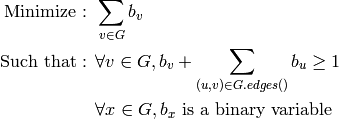
Returns a minimum dominating set of the graph represented by the list of its vertices. For more information, see the Wikipedia article on dominating sets.
A minimum dominating set  of a graph is
a set of its vertices of minimal cardinality such
that any vertex of is in or has one of its neighbors
in .
of a graph is
a set of its vertices of minimal cardinality such
that any vertex of is in or has one of its neighbors
in .
As an optimization problem, it can be expressed as:
INPUT:
EXAMPLES:
A basic illustration on a PappusGraph:
sage: g=graphs.PappusGraph()
sage: g.dominating_set(value_only=True)
5.0
If we build a graph from two disjoint stars, then link their centers we will find a difference between the cardinality of an independent set and a stable independent set:
sage: g = 2 * graphs.StarGraph(5)
sage: g.add_edge(0,6)
sage: len(g.dominating_set())
2
sage: len(g.dominating_set(independent=True))
6
Return the eccentricity of vertex (or vertices) v.
The eccentricity of a vertex is the maximum distance to any other vertex.
INPUT:
EXAMPLES:
sage: G = graphs.KrackhardtKiteGraph()
sage: G.eccentricity()
[4, 4, 4, 4, 4, 3, 3, 2, 3, 4]
sage: G.vertices()
[0, 1, 2, 3, 4, 5, 6, 7, 8, 9]
sage: G.eccentricity(7)
2
sage: G.eccentricity([7,8,9])
[3, 4, 2]
sage: G.eccentricity([7,8,9], with_labels=True) == {8: 3, 9: 4, 7: 2}
True
sage: G = Graph( { 0 : [], 1 : [], 2 : [1] } )
sage: G.eccentricity()
[+Infinity, +Infinity, +Infinity]
sage: G = Graph({0:[]})
sage: G.eccentricity(with_labels=True)
{0: 0}
sage: G = Graph({0:[], 1:[]})
sage: G.eccentricity(with_labels=True)
{0: +Infinity, 1: +Infinity}
Returns a list of edges  with in vertices1
and in vertices2. If vertices2 is None, then
it is set to the complement of vertices1.
with in vertices1
and in vertices2. If vertices2 is None, then
it is set to the complement of vertices1.
In a digraph, the external boundary of a vertex are those
vertices with an arc  .
.
INPUT:
 of
vertices.
of
vertices.EXAMPLES:
sage: K = graphs.CompleteBipartiteGraph(9,3)
sage: len(K.edge_boundary( [0,1,2,3,4,5,6,7,8], [9,10,11] ))
27
sage: K.size()
27
Note that the edge boundary preserves direction:
sage: K = graphs.CompleteBipartiteGraph(9,3).to_directed()
sage: len(K.edge_boundary( [0,1,2,3,4,5,6,7,8], [9,10,11] ))
27
sage: K.size()
54
sage: D = DiGraph({0:[1,2], 3:[0]})
sage: D.edge_boundary([0])
[(0, 1, None), (0, 2, None)]
sage: D.edge_boundary([0], labels=False)
[(0, 1), (0, 2)]
TESTS:
sage: G = graphs.DiamondGraph()
sage: G.edge_boundary([0,1])
[(0, 2, {}), (1, 2, {}), (1, 3, {})]
sage: G = graphs.PetersenGraph()
sage: G.edge_boundary([0], [0])
[]
Returns the edge connectivity of the graph. For more information, see the Wikipedia article on connectivity.
INPUT:
 is assumed.).
EXAMPLES:
A basic application on the PappusGraph:
sage: g = graphs.PappusGraph()
sage: g.edge_connectivity()
3.0
The edge connectivity of a complete graph ( and of a random graph ) is its minimum degree, and one of the two parts of the bipartition is reduced to only one vertex. The cutedges isomorphic to a Star graph:
sage: g = graphs.CompleteGraph(5)
sage: [ value, edges, [ setA, setB ]] = g.edge_connectivity(vertices=True)
sage: print value
4.0
sage: len(setA) == 1 or len(setB) == 1
True
sage: cut = Graph()
sage: cut.add_edges(edges)
sage: cut.is_isomorphic(graphs.StarGraph(4))
True
Even if obviously in any graph we know that the edge connectivity is less than the minimum degree of the graph:
sage: g = graphs.RandomGNP(10,.3)
sage: min(g.degree()) >= g.edge_connectivity()
True
If we build a tree then assign to its edges a random value, the minimum cut will be the edge with minimum value:
sage: g = graphs.RandomGNP(15,.5)
sage: tree = Graph()
sage: tree.add_edges(g.min_spanning_tree())
sage: for u,v in tree.edge_iterator(labels=None):
...        tree.set_edge_label(u,v,random())
sage: minimum = min([l for u,v,l in tree.edge_iterator()])
sage: [value, [(u,v,l)]] = tree.edge_connectivity(value_only=False, use_edge_labels=True)
sage: l == minimum
True
When value_only = True, this function is optimized for small connexity values and does not need to build a linear program.
It is the case for connected graphs which are not connected
sage: g = 2 * graphs.PetersenGraph()
sage: g.edge_connectivity()
0.0
Or if they are just 1-connected
sage: g = graphs.PathGraph(10)
sage: g.edge_connectivity()
1.0
For directed graphs, the strong connexity is tested through the dedicated function
sage: g = digraphs.ButterflyGraph(3)
sage: g.edge_connectivity()
0.0
Returns a minimum edge cut between vertices and  represented by a list of edges.
A minimum edge cut between two vertices and of self
is a set  of edges of minimum weight such that the graph
obtained by removing from self is disconnected. For more
information, see the
Wikipedia article on cuts.
of edges of minimum weight such that the graph
obtained by removing from self is disconnected. For more
information, see the
Wikipedia article on cuts.
INPUT:
is assumed). Otherwise, each edge has weight .OUTPUT:
Real number or tuple, depending on the given arguments (examples are given below).
EXAMPLES:
A basic application in the Pappus graph:
sage: g = graphs.PappusGraph()
sage: g.edge_cut(1, 2, value_only=True)
3.0
If the graph is a path with randomly weighted edges:
sage: g = graphs.PathGraph(15)
sage: for (u,v) in g.edge_iterator(labels=None):
...      g.set_edge_label(u,v,random())
The edge cut between the two ends is the edge of minimum weight:
sage: minimum = min([l for u,v,l in g.edge_iterator()])
sage: abs(minimum - g.edge_cut(0, 14, use_edge_labels=True)) < 10**(-5)
True
sage: [value,[[u,v]]] = g.edge_cut(0, 14, use_edge_labels=True, value_only=False)
sage: g.edge_label(u, v) == minimum
True
The two sides of the edge cut are obviously shorter paths:
sage: value,edges,[set1,set2] = g.edge_cut(0, 14, use_edge_labels=True, vertices=True)
sage: g.subgraph(set1).is_isomorphic(graphs.PathGraph(len(set1)))
True
sage: g.subgraph(set2).is_isomorphic(graphs.PathGraph(len(set2)))
True
sage: len(set1) + len(set2) == g.order()
True
Returns a list of edge-disjoint paths between two vertices as given by Menger’s theorem.
The edge version of Menger’s theorem asserts that the size
of the minimum edge cut between two vertices and`t`
(the minimum number of edges whose removal disconnects
and ) is equal to the maximum number of pairwise
edge-independent paths from to .
This function returns a list of such paths.
Note
This function is topological : it does not take the eventual weights of the edges into account.
EXAMPLE:
In a complete bipartite graph
sage: g = graphs.CompleteBipartiteGraph(2,3)
sage: g.edge_disjoint_paths(0,1)
[[0, 2, 1], [0, 3, 1], [0, 4, 1]]
Returns the desired number of edge-disjoint spanning trees/arborescences.
INPUT:
ALGORITHM:
Mixed Integer Linear Program. The formulation can be found in [JVNC].
There are at least two possible rewritings of this method which do not use Linear Programming:
- The algorithm presented in the paper entitled “A short proof of the tree-packing theorem”, by Thomas Kaiser [KaisPacking].
- The implementation of a Matroid class and of the Matroid Union Theorem (see section 42.3 of [SchrijverCombOpt]), applied to the cycle Matroid (see chapter 51 of [SchrijverCombOpt]).
EXAMPLES:
The Petersen Graph does have a spanning tree (it is connected):
sage: g = graphs.PetersenGraph()
sage: [T] = g.edge_disjoint_spanning_trees(1)
sage: T.is_tree()
True
Though, it does not have 2 edge-disjoint trees (as it has less
than  edges):
sage: g.edge_disjoint_spanning_trees(2)
...
ValueError: This graph does not contain the required number of trees/arborescences !
By Edmond’s theorem, a graph which is -connected always has edge-disjoint
arborescences, regardless of the root we pick:
sage: g = digraphs.RandomDirectedGNP(30,.3)
sage: k = Integer(g.edge_connectivity())
sage: arborescences = g.edge_disjoint_spanning_trees(k)
sage: all([a.is_directed_acyclic() for a in arborescences])
True
sage: all([a.is_connected() for a in arborescences])
True
In the undirected case, we can only ensure half of it:
sage: g = graphs.RandomGNP(30,.3)
sage: k = floor(Integer(g.edge_connectivity())/2)
sage: trees = g.edge_disjoint_spanning_trees(k)
sage: all([t.is_tree() for t in trees])
True
REFERENCES:
| [JVNC] | David Joyner, Minh Van Nguyen, and Nathann Cohen, Algorithmic Graph Theory, http://code.google.com/p/graph-theory-algorithms-book/ |
| [KaisPacking] | Thomas Kaiser A short proof of the tree-packing theorem http://arxiv.org/abs/0911.2809 |
| [SchrijverCombOpt] | (1, 2) Alexander Schrijver Combinatorial optimization: polyhedra and efficiency 2003 |
Returns an iterator over the edges incident with any vertex given. If the graph is directed, iterates over edges going out only. If vertices is None, then returns an iterator over all edges. If self is directed, returns outgoing edges only.
INPUT:
EXAMPLES:
sage: for i in graphs.PetersenGraph().edge_iterator([0]):
...    print i
(0, 1, None)
(0, 4, None)
(0, 5, None)
sage: D = DiGraph( { 0 : [1,2], 1: [0] } )
sage: for i in D.edge_iterator([0]):
...    print i
(0, 1, None)
(0, 2, None)
sage: G = graphs.TetrahedralGraph()
sage: list(G.edge_iterator(labels=False))
[(0, 1), (0, 2), (0, 3), (1, 2), (1, 3), (2, 3)]
sage: D = DiGraph({1:[0], 2:[0]})
sage: list(D.edge_iterator(0))
[]
sage: list(D.edge_iterator(0, ignore_direction=True))
[(1, 0, None), (2, 0, None)]
Returns the label of an edge. Note that if the graph allows multiple edges, then a list of labels on the edge is returned.
EXAMPLES:
sage: G = Graph({0 : {1 : 'edgelabel'}}, sparse=True)
sage: G.edges(labels=False)
[(0, 1)]
sage: G.edge_label( 0, 1 )
'edgelabel'
sage: D = DiGraph({0 : {1 : 'edgelabel'}}, sparse=True)
sage: D.edges(labels=False)
[(0, 1)]
sage: D.edge_label( 0, 1 )
'edgelabel'
sage: G = Graph(multiedges=True, sparse=True)
sage: [G.add_edge(0,1,i) for i in range(1,6)]
[None, None, None, None, None]
sage: sorted(G.edge_label(0,1))
[1, 2, 3, 4, 5]
Returns a list of edge labels.
EXAMPLES:
sage: G = Graph({0:{1:'x',2:'z',3:'a'}, 2:{5:'out'}}, sparse=True)
sage: G.edge_labels()
['x', 'z', 'a', 'out']
sage: G = DiGraph({0:{1:'x',2:'z',3:'a'}, 2:{5:'out'}}, sparse=True)
sage: G.edge_labels()
['x', 'z', 'a', 'out']
Return a list of edges. Each edge is a triple (u,v,l) where u and v are vertices and l is a label.
INPUT:
OUTPUT: A list of tuples. It is safe to change the returned list.
EXAMPLES:
sage: graphs.DodecahedralGraph().edges()
[(0, 1, {}), (0, 10, {}), (0, 19, {}), (1, 2, {}), (1, 8, {}), (2, 3, {}), (2, 6, {}), (3, 4, {}), (3, 19, {}), (4, 5, {}), (4, 17, {}), (5, 6, {}), (5, 15, {}), (6, 7, {}), (7, 8, {}), (7, 14, {}), (8, 9, {}), (9, 10, {}), (9, 13, {}), (10, 11, {}), (11, 12, {}), (11, 18, {}), (12, 13, {}), (12, 16, {}), (13, 14, {}), (14, 15, {}), (15, 16, {}), (16, 17, {}), (17, 18, {}), (18, 19, {})]
sage: graphs.DodecahedralGraph().edges(labels=False)
[(0, 1), (0, 10), (0, 19), (1, 2), (1, 8), (2, 3), (2, 6), (3, 4), (3, 19), (4, 5), (4, 17), (5, 6), (5, 15), (6, 7), (7, 8), (7, 14), (8, 9), (9, 10), (9, 13), (10, 11), (11, 12), (11, 18), (12, 13), (12, 16), (13, 14), (14, 15), (15, 16), (16, 17), (17, 18), (18, 19)]
sage: D = graphs.DodecahedralGraph().to_directed()
sage: D.edges()
[(0, 1, {}), (0, 10, {}), (0, 19, {}), (1, 0, {}), (1, 2, {}), (1, 8, {}), (2, 1, {}), (2, 3, {}), (2, 6, {}), (3, 2, {}), (3, 4, {}), (3, 19, {}), (4, 3, {}), (4, 5, {}), (4, 17, {}), (5, 4, {}), (5, 6, {}), (5, 15, {}), (6, 2, {}), (6, 5, {}), (6, 7, {}), (7, 6, {}), (7, 8, {}), (7, 14, {}), (8, 1, {}), (8, 7, {}), (8, 9, {}), (9, 8, {}), (9, 10, {}), (9, 13, {}), (10, 0, {}), (10, 9, {}), (10, 11, {}), (11, 10, {}), (11, 12, {}), (11, 18, {}), (12, 11, {}), (12, 13, {}), (12, 16, {}), (13, 9, {}), (13, 12, {}), (13, 14, {}), (14, 7, {}), (14, 13, {}), (14, 15, {}), (15, 5, {}), (15, 14, {}), (15, 16, {}), (16, 12, {}), (16, 15, {}), (16, 17, {}), (17, 4, {}), (17, 16, {}), (17, 18, {}), (18, 11, {}), (18, 17, {}), (18, 19, {}), (19, 0, {}), (19, 3, {}), (19, 18, {})]
sage: D.edges(labels = False)
[(0, 1), (0, 10), (0, 19), (1, 0), (1, 2), (1, 8), (2, 1), (2, 3), (2, 6), (3, 2), (3, 4), (3, 19), (4, 3), (4, 5), (4, 17), (5, 4), (5, 6), (5, 15), (6, 2), (6, 5), (6, 7), (7, 6), (7, 8), (7, 14), (8, 1), (8, 7), (8, 9), (9, 8), (9, 10), (9, 13), (10, 0), (10, 9), (10, 11), (11, 10), (11, 12), (11, 18), (12, 11), (12, 13), (12, 16), (13, 9), (13, 12), (13, 14), (14, 7), (14, 13), (14, 15), (15, 5), (15, 14), (15, 16), (16, 12), (16, 15), (16, 17), (17, 4), (17, 16), (17, 18), (18, 11), (18, 17), (18, 19), (19, 0), (19, 3), (19, 18)]
Returns a list of edges incident with any vertex given. If vertices is None, returns a list of all edges in graph. For digraphs, only lists outward edges.
INPUT:
EXAMPLES:
sage: graphs.PetersenGraph().edges_incident([0,9], labels=False)
[(0, 1), (0, 4), (0, 5), (4, 9), (6, 9), (7, 9)]
sage: D = DiGraph({0:[1]})
sage: D.edges_incident([0])
[(0, 1, None)]
sage: D.edges_incident([1])
[]
Returns the right eigenspaces of the adjacency matrix of the graph.
INPUT:
OUTPUT:
A list of pairs. Each pair is an eigenvalue of the adjacency matrix of the graph, followed by the vector space that is the eigenspace for that eigenvalue, when the eigenvectors are placed on the right of the matrix.
For some graphs, some of the the eigenspaces are described exactly by vector spaces over a NumberField. For numerical eigenvectors use eigenvectors().
EXAMPLES:
sage: P = graphs.PetersenGraph()
sage: P.eigenspaces()
[
(3, Vector space of degree 10 and dimension 1 over Rational Field
User basis matrix:
[1 1 1 1 1 1 1 1 1 1]),
(-2, Vector space of degree 10 and dimension 4 over Rational Field
User basis matrix:
[ 1  0  0  0 -1 -1 -1  0  1  1]
[ 0  1  0  0 -1  0 -2 -1  1  2]
[ 0  0  1  0 -1  1 -1 -2  0  2]
[ 0  0  0  1 -1  1  0 -1 -1  1]),
(1, Vector space of degree 10 and dimension 5 over Rational Field
User basis matrix:
[ 1  0  0  0  0  1 -1  0  0 -1]
[ 0  1  0  0  0 -1  1 -1  0  0]
[ 0  0  1  0  0  0 -1  1 -1  0]
[ 0  0  0  1  0  0  0 -1  1 -1]
[ 0  0  0  0  1 -1  0  0 -1  1])
]
Eigenspaces for the Laplacian should be identical since the Petersen graph is regular. However, since the output also contains the eigenvalues, the two outputs are slightly different.
sage: P.eigenspaces(laplacian=True)
[
(0, Vector space of degree 10 and dimension 1 over Rational Field
User basis matrix:
[1 1 1 1 1 1 1 1 1 1]),
(5, Vector space of degree 10 and dimension 4 over Rational Field
User basis matrix:
[ 1  0  0  0 -1 -1 -1  0  1  1]
[ 0  1  0  0 -1  0 -2 -1  1  2]
[ 0  0  1  0 -1  1 -1 -2  0  2]
[ 0  0  0  1 -1  1  0 -1 -1  1]),
(2, Vector space of degree 10 and dimension 5 over Rational Field
User basis matrix:
[ 1  0  0  0  0  1 -1  0  0 -1]
[ 0  1  0  0  0 -1  1 -1  0  0]
[ 0  0  1  0  0  0 -1  1 -1  0]
[ 0  0  0  1  0  0  0 -1  1 -1]
[ 0  0  0  0  1 -1  0  0 -1  1])
]
Notice how one eigenspace below is described with a square root of 2. For the two possible values (positive and negative) there is a corresponding eigenspace.
sage: C = graphs.CycleGraph(8)
sage: C.eigenspaces()
[
(2, Vector space of degree 8 and dimension 1 over Rational Field
User basis matrix:
[1 1 1 1 1 1 1 1]),
(-2, Vector space of degree 8 and dimension 1 over Rational Field
User basis matrix:
[ 1 -1  1 -1  1 -1  1 -1]),
(0, Vector space of degree 8 and dimension 2 over Rational Field
User basis matrix:
[ 1  0 -1  0  1  0 -1  0]
[ 0  1  0 -1  0  1  0 -1]),
(a3, Vector space of degree 8 and dimension 2 over Number Field in a3 with defining polynomial x^2 - 2
User basis matrix:
[  1   0  -1 -a3  -1   0   1  a3]
[  0   1  a3   1   0  -1 -a3  -1])
]
A digraph may have complex eigenvalues and eigenvectors. For a 3-cycle, we have:
sage: T = DiGraph({0:[1], 1:[2], 2:[0]})
sage: T.eigenspaces()
[
(1, Vector space of degree 3 and dimension 1 over Rational Field
User basis matrix:
[1 1 1]),
(a1, Vector space of degree 3 and dimension 1 over Number Field in a1 with defining polynomial x^2 + x + 1
User basis matrix:
[      1      a1 -a1 - 1])
]
Returns the right eigenvectors of the adjacency matrix of the graph.
INPUT:
OUTPUT:
A list of triples. Each triple begins with an eigenvalue of the adjacency matrix of the graph. This is followed by a list of eigenvectors for the eigenvalue, when the eigenvectors are placed on the right side of the matrix. Together, the eigenvectors form a basis for the eigenspace. The triple concludes with the algebraic multiplicity of the eigenvalue.
For some graphs, the exact eigenspaces provided by eigenspaces() provide additional insight into the structure of the eigenspaces.
EXAMPLES:
sage: P = graphs.PetersenGraph()
sage: P.eigenvectors()
[(3, [
(1, 1, 1, 1, 1, 1, 1, 1, 1, 1)
], 1), (-2, [
(1, 0, 0, 0, -1, -1, -1, 0, 1, 1),
(0, 1, 0, 0, -1, 0, -2, -1, 1, 2),
(0, 0, 1, 0, -1, 1, -1, -2, 0, 2),
(0, 0, 0, 1, -1, 1, 0, -1, -1, 1)
], 4), (1, [
(1, 0, 0, 0, 0, 1, -1, 0, 0, -1),
(0, 1, 0, 0, 0, -1, 1, -1, 0, 0),
(0, 0, 1, 0, 0, 0, -1, 1, -1, 0),
(0, 0, 0, 1, 0, 0, 0, -1, 1, -1),
(0, 0, 0, 0, 1, -1, 0, 0, -1, 1)
], 5)]
Eigenspaces for the Laplacian should be identical since the Petersen graph is regular. However, since the output also contains the eigenvalues, the two outputs are slightly different.
sage: P.eigenvectors(laplacian=True)
[(0, [
(1, 1, 1, 1, 1, 1, 1, 1, 1, 1)
], 1), (5, [
(1, 0, 0, 0, -1, -1, -1, 0, 1, 1),
(0, 1, 0, 0, -1, 0, -2, -1, 1, 2),
(0, 0, 1, 0, -1, 1, -1, -2, 0, 2),
(0, 0, 0, 1, -1, 1, 0, -1, -1, 1)
], 4), (2, [
(1, 0, 0, 0, 0, 1, -1, 0, 0, -1),
(0, 1, 0, 0, 0, -1, 1, -1, 0, 0),
(0, 0, 1, 0, 0, 0, -1, 1, -1, 0),
(0, 0, 0, 1, 0, 0, 0, -1, 1, -1),
(0, 0, 0, 0, 1, -1, 0, 0, -1, 1)
], 5)]
sage: C = graphs.CycleGraph(8)
sage: C.eigenvectors()
[(2, [
(1, 1, 1, 1, 1, 1, 1, 1)
], 1), (-2, [
(1, -1, 1, -1, 1, -1, 1, -1)
], 1), (0, [
(1, 0, -1, 0, 1, 0, -1, 0),
(0, 1, 0, -1, 0, 1, 0, -1)
], 2), (-1.4142135623..., [(1, 0, -1, 1.4142135623..., -1, 0, 1, -1.4142135623...), (0, 1, -1.4142135623..., 1, 0, -1, 1.4142135623..., -1)], 2), (1.4142135623..., [(1, 0, -1, -1.4142135623..., -1, 0, 1, 1.4142135623...), (0, 1, 1.4142135623..., 1, 0, -1, -1.4142135623..., -1)], 2)]
A digraph may have complex eigenvalues. Previously, the complex parts of graph eigenvalues were being dropped. For a 3-cycle, we have:
sage: T = DiGraph({0:[1], 1:[2], 2:[0]})
sage: T.eigenvectors()
[(1, [
(1, 1, 1)
], 1), (-0.5000000000... - 0.8660254037...*I, [(1, -0.5000000000... - 0.8660254037...*I, -0.5000000000... + 0.8660254037...*I)], 1), (-0.5000000000... + 0.8660254037...*I, [(1, -0.5000000000... + 0.8660254037...*I, -0.5000000000... - 0.8660254037...*I)], 1)]
Returns a DiGraph which is an eulerian orientation of the current graph.
An eulerian graph being a graph such that any vertex has an even degree,
an eulerian orientation of a graph is an orientation of its edges such
that each vertex verifies  , where
  and
and
 respectively represent the out-degree and the in-degree of a vertex.
If the graph is not eulerian, the orientation verifies for any vertex
that  .
.
ALGORITHM:
This algorithm is a random walk through the edges of the graph, which orients the edges according to the walk. When a vertex is reached which has no non-oriented edge ( this vertex must have odd degree ), the walk resumes at another vertex of odd degree, if any.
This algorithm has complexity , where  is the number of edges
in the graph.
is the number of edges
in the graph.
EXAMPLES:
The CubeGraph with parameter 4, which is regular of even degree, has an
eulerian orientation such that  :
:
sage: g=graphs.CubeGraph(4)
sage: g.degree()
[4, 4, 4, 4, 4, 4, 4, 4, 4, 4, 4, 4, 4, 4, 4, 4]
sage: o=g.eulerian_orientation()
sage: o.in_degree()
[2, 2, 2, 2, 2, 2, 2, 2, 2, 2, 2, 2, 2, 2, 2, 2]
sage: o.out_degree()
[2, 2, 2, 2, 2, 2, 2, 2, 2, 2, 2, 2, 2, 2, 2, 2]
Secondly, the Petersen Graph, which is 3 regular has an orientation
such that the difference between and is at most 1:
sage: g=graphs.PetersenGraph()
sage: o=g.eulerian_orientation()
sage: o.in_degree()
[2, 2, 2, 2, 2, 1, 1, 1, 1, 1]
sage: o.out_degree()
[1, 1, 1, 1, 1, 2, 2, 2, 2, 2]
Returns a maximum flow in the graph from x to y represented by an optimal valuation of the edges. For more information, see the Wikipedia article on maximum flow.
As an optimization problem, is can be expressed this way :
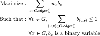
INPUT:
is assumed.). to (useful for vertex
connectivity parameters).
to (useful for vertex
connectivity parameters).EXAMPLES:
Two basic applications of the flow method for the PappusGraph and the
ButterflyGraph with parameter
sage: g=graphs.PappusGraph()
sage: g.flow(1,2)
3.0
sage: b=digraphs.ButterflyGraph(2)
sage: b.flow(('00',1),('00',2))
1.0
The flow method can be used to compute a matching in a bipartite graph
by linking a source to all the vertices of the first set and linking
a sink to all the vertices of the second set, then computing
a maximum  flow
flow
sage: g = DiGraph()
sage: g.add_edges([('s',i) for i in range(4)])
sage: g.add_edges([(i,4+j) for i in range(4) for j in range(4)])
sage: g.add_edges([(4+i,'t') for i in range(4)])
sage: [cardinal, flow_graph] = g.flow('s','t',integer=True,value_only=False)
sage: flow_graph.delete_vertices(['s','t'])
sage: len(flow_graph.edges(labels=None))
4
Returns the minimal genus of the graph. The genus of a compact surface is the number of handles it has. The genus of a graph is the minimal genus of the surface it can be embedded into.
Note - This function uses Euler’s formula and thus it is necessary to consider only connected graphs.
INPUT:
EXAMPLES:
sage: g = graphs.PetersenGraph()
sage: g.genus() # tests for minimal genus by default
1
sage: g.genus(on_embedding=True, maximal=True) # on_embedding overrides minimal and maximal arguments
1
sage: g.genus(maximal=True) # setting maximal to True overrides default minimal=True
3
sage: g.genus(on_embedding=g.get_embedding()) # can also send a valid combinatorial embedding dict
3
sage: (graphs.CubeGraph(3)).genus()
0
sage: K23 = graphs.CompleteBipartiteGraph(2,3)
sage: K23.genus()
0
sage: K33 = graphs.CompleteBipartiteGraph(3,3)
sage: K33.genus()
1
Using the circular argument, we can compute the minimal genus preserving a planar, ordered boundary:
sage: cube = graphs.CubeGraph(2)
sage: cube.set_boundary(['01','10'])
sage: cube.genus()
0
sage: cube.is_circular_planar()
True
sage: cube.genus(circular=True)
0
sage: cube.genus(circular=True, on_embedding=True)
0
sage: cube.genus(circular=True, maximal=True)
...
NotImplementedError: Cannot compute the maximal genus of a genus respecting a boundary.
Note: not everything works for multigraphs, looped graphs or digraphs. But the minimal genus is ultimately computable for every connected graph – but the embedding we obtain for the simple graph can’t be easily converted to an embedding of a non-simple graph. Also, the maximal genus of a multigraph does not trivially correspond to that of its simple graph.
sage: G = DiGraph({ 0 : [0,1,1,1], 1 : [2,2,3,3], 2 : [1,3,3], 3:[0,3]}) sage: G.genus() Traceback (most recent call last): ... NotImplementedError: Can’t work with embeddings of non-simple graphs sage: G.to_simple().genus() 0 sage: G.genus(set_embedding=False) 0 sage: G.genus(maximal=True, set_embedding=False) Traceback (most recent call last): ... NotImplementedError: Can’t compute the maximal genus of a graph with loops or multiple edges
Returns the boundary of the (di)graph.
EXAMPLES:
sage: G = graphs.PetersenGraph()
sage: G.set_boundary([0,1,2,3,4])
sage: G.get_boundary()
[0, 1, 2, 3, 4]
Returns the attribute _embedding if it exists. _embedding is a dictionary organized with vertex labels as keys and a list of each vertex’s neighbors in clockwise order.
Error-checked to insure valid embedding is returned.
EXAMPLES:
sage: G = graphs.PetersenGraph()
sage: G.genus()
1
sage: G.get_embedding()
{0: [1, 4, 5], 1: [0, 2, 6], 2: [1, 3, 7], 3: [2, 4, 8], 4: [0, 3, 9], 5: [0, 7, 8], 6: [1, 9, 8], 7: [2, 5, 9], 8: [3, 6, 5], 9: [4, 6, 7]}
Returns the position dictionary, a dictionary specifying the coordinates of each vertex.
EXAMPLES: By default, the position of a graph is None:
sage: G = Graph()
sage: G.get_pos()
sage: G.get_pos() is None
True
sage: P = G.plot(save_pos=True)
sage: G.get_pos()
{}
Some of the named graphs come with a pre-specified positioning:
sage: G = graphs.PetersenGraph()
sage: G.get_pos()
{0: (..., ...),
 ...
 9: (..., ...)}
Retrieve the object associated with a given vertex.
INPUT:
EXAMPLES:
sage: d = {0 : graphs.DodecahedralGraph(), 1 : graphs.FlowerSnark(), 2 : graphs.MoebiusKantorGraph(), 3 : graphs.PetersenGraph() }
sage: d[2]
Moebius-Kantor Graph: Graph on 16 vertices
sage: T = graphs.TetrahedralGraph()
sage: T.vertices()
[0, 1, 2, 3]
sage: T.set_vertices(d)
sage: T.get_vertex(1)
Flower Snark: Graph on 20 vertices
Return a dictionary of the objects associated to each vertex.
INPUT:
EXAMPLES:
sage: d = {0 : graphs.DodecahedralGraph(), 1 : graphs.FlowerSnark(), 2 : graphs.MoebiusKantorGraph(), 3 : graphs.PetersenGraph() }
sage: T = graphs.TetrahedralGraph()
sage: T.set_vertices(d)
sage: T.get_vertices([1,2])
{1: Flower Snark: Graph on 20 vertices,
 2: Moebius-Kantor Graph: Graph on 16 vertices}
Computes the girth of the graph. For directed graphs, computes the girth of the undirected graph.
The girth is the length of the shortest cycle in the graph. Graphs without cycles have infinite girth.
EXAMPLES:
sage: graphs.TetrahedralGraph().girth()
3
sage: graphs.CubeGraph(3).girth()
4
sage: graphs.PetersenGraph().girth()
5
sage: graphs.HeawoodGraph().girth()
6
sage: graphs.trees(9).next().girth()
+Infinity
Returns a GraphPlot object.
EXAMPLES:
Creating a graphplot object uses the same options as graph.plot():
sage: g = Graph({}, loops=True, multiedges=True, sparse=True)
sage: g.add_edges([(0,0,'a'),(0,0,'b'),(0,1,'c'),(0,1,'d'),
...     (0,1,'e'),(0,1,'f'),(0,1,'f'),(2,1,'g'),(2,2,'h')])
sage: g.set_boundary([0,1])
sage: GP = g.graphplot(edge_labels=True, color_by_label=True, edge_style='dashed')
sage: GP.plot()
We can modify the graphplot object. Notice that the changes are cumulative:
sage: GP.set_edges(edge_style='solid')
sage: GP.plot()
sage: GP.set_vertices(talk=True)
sage: GP.plot()
Returns a representation in the dot language.
The dot language is a text based format for graphs. It is used by the software suite graphviz. The specifications of the language are available on the web (see the reference [dotspec]).
INPUT:
EXAMPLES:
sage: G = Graph({0:{1:None,2:None}, 1:{0:None,2:None}, 2:{0:None,1:None,3:'foo'}, 3:{2:'foo'}},sparse=True)
sage: print G.graphviz_string(edge_labels=True)
graph {
  "0" [label="0"];
  "1" [label="1"];
  "2" [label="2"];
  "3" [label="3"];
<BLANKLINE>
  "0" -- "1";
  "0" -- "2";
  "1" -- "2";
  "2" -- "3" [label="foo"];
}
A variant, with the labels in latex, for post-processing with dot2tex:
sage: print G.graphviz_string(edge_labels=True,labels = "latex")
graph {
  node [shape="plaintext"];
  "0" [label=" ", texlbl="$0$"];
  "1" [label=" ", texlbl="$1$"];
  "2" [label=" ", texlbl="$2$"];
  "3" [label=" ", texlbl="$3$"];
<BLANKLINE>
  "0" -- "1";
  "0" -- "2";
  "1" -- "2";
  "2" -- "3" [label=" ", texlbl="$\texttt{foo}$"];
}
Same, with a digraph and a color for edges:
sage: G = DiGraph({0:{1:None,2:None}, 1:{2:None}, 2:{3:'foo'}, 3:{}} ,sparse=True)
sage: print G.graphviz_string(edge_color="red")
digraph {
  "0" [label="0"];
  "1" [label="1"];
  "2" [label="2"];
  "3" [label="3"];
<BLANKLINE>
  edge [color="red"];
  "0" -> "1";
  "0" -> "2";
  "1" -> "2";
  "2" -> "3";
}
A digraph using latex labels for vertices and edges:
sage: f(x) = -1/x
sage: g(x) = 1/(x+1)
sage: G = DiGraph()
sage: G.add_edges([(i,f(i),f) for i in (1,2,1/2,1/4)])
sage: G.add_edges([(i,g(i),g) for i in (1,2,1/2,1/4)])
sage: print G.graphviz_string(labels="latex",edge_labels=True)
digraph {
  node [shape="plaintext"];
  "2/3" [label=" ", texlbl="$\frac{2}{3}$"];
  "1/3" [label=" ", texlbl="$\frac{1}{3}$"];
  "1/2" [label=" ", texlbl="$\frac{1}{2}$"];
  "1" [label=" ", texlbl="$1$"];
  "1/4" [label=" ", texlbl="$\frac{1}{4}$"];
  "4/5" [label=" ", texlbl="$\frac{4}{5}$"];
  "-4" [label=" ", texlbl="$-4$"];
  "2" [label=" ", texlbl="$2$"];
  "-2" [label=" ", texlbl="$-2$"];
  "-1/2" [label=" ", texlbl="$-\frac{1}{2}$"];
  "-1" [label=" ", texlbl="$-1$"];
<BLANKLINE>
  "1/2" -> "-2" [label=" ", texlbl="$x \ {\mapsto}\ \frac{-1}{x}$"];
  "1/2" -> "2/3" [label=" ", texlbl="$x \ {\mapsto}\ \frac{1}{x + 1}$"];
  "1" -> "-1" [label=" ", texlbl="$x \ {\mapsto}\ \frac{-1}{x}$"];
  "1" -> "1/2" [label=" ", texlbl="$x \ {\mapsto}\ \frac{1}{x + 1}$"];
  "1/4" -> "-4" [label=" ", texlbl="$x \ {\mapsto}\ \frac{-1}{x}$"];
  "1/4" -> "4/5" [label=" ", texlbl="$x \ {\mapsto}\ \frac{1}{x + 1}$"];
  "2" -> "-1/2" [label=" ", texlbl="$x \ {\mapsto}\ \frac{-1}{x}$"];
  "2" -> "1/3" [label=" ", texlbl="$x \ {\mapsto}\ \frac{1}{x + 1}$"];
}
TESTS:
The following digraph has tuples as vertices:
sage: print digraphs.ButterflyGraph(1).graphviz_string()
digraph {
  "1,1" [label="('1', 1)"];
  "0,0" [label="('0', 0)"];
  "1,0" [label="('1', 0)"];
  "0,1" [label="('0', 1)"];
<BLANKLINE>
  "0,0" -> "1,1";
  "0,0" -> "0,1";
  "1,0" -> "1,1";
  "1,0" -> "0,1";
}
The following digraph has vertices with newlines in their string representations:
sage: m1 = matrix(3,3)
sage: m2 = matrix(3,3, 1)
sage: m1.set_immutable()
sage: m2.set_immutable()
sage: g = DiGraph({ m1: [m2] })
sage: print g.graphviz_string()
digraph {
  "000000000" [label="[0 0 0]\n\
  [0 0 0]\n\
  [0 0 0]"];
  "100010001" [label="[1 0 0]\n\
  [0 1 0]\n\
  [0 0 1]"];
<BLANKLINE>
  "000000000" -> "100010001";
}
REFERENCES:
| [dotspec] | http://www.graphviz.org/doc/info/lang.html |
Write a representation in the dot in a file.
The dot language is a plaintext format for graph structures. See the documentation of graphviz_string() for available options.
INPUT:
filename - the name of the file to write in
options - options for the graphviz string
EXAMPLES:
sage: G = Graph({0:{1:None,2:None}, 1:{0:None,2:None}, 2:{0:None,1:None,3:'foo'}, 3:{2:'foo'}},sparse=True)
sage: G.graphviz_to_file_named(os.environ['SAGE_TESTDIR']+'/temp_graphviz',edge_labels=True)
sage: print open(os.environ['SAGE_TESTDIR']+'/temp_graphviz').read()
graph {
  "0" [label="0"];
  "1" [label="1"];
  "2" [label="2"];
  "3" [label="3"];
<BLANKLINE>
  "0" -- "1";
  "0" -- "2";
  "1" -- "2";
  "2" -- "3" [label="foo"];
}
Returns a hamiltonian cycle/circuit of the current graph/digraph
A graph (resp. digraph) is said to be hamiltonian if it contains as a subgraph a cycle (resp. a circuit) going through all the vertices.
Computing a hamiltonian cycle/circuit being NP-Complete, this algorithm could run for some time depending on the instance.
ALGORITHM:
See Graph.traveling_salesman_problem.
OUTPUT:
Returns a hamiltonian cycle/circuit if it exists. Otherwise, raises a ValueError exception.
NOTE:
This function, as is_hamiltonian, computes a hamiltonian cycle if it exists : the user should NOT test for hamiltonicity using is_hamiltonian before calling this function, as it would result in computing it twice.
EXAMPLES:
The Heawood Graph is known to be hamiltonian
sage: g = graphs.HeawoodGraph()
sage: g.hamiltonian_cycle()
TSP from Heawood graph: Graph on 14 vertices
The Petergraph, though, is not
sage: g = graphs.PetersenGraph()
sage: g.hamiltonian_cycle()
...
ValueError: The given graph is not hamiltonian
Returns True if (u, v) is an edge, False otherwise.
INPUT: The following forms are accepted by NetworkX:
EXAMPLES:
sage: graphs.EmptyGraph().has_edge(9,2)
False
sage: DiGraph().has_edge(9,2)
False
sage: G = Graph(sparse=True)
sage: G.add_edge(0,1,"label")
sage: G.has_edge(0,1,"different label")
False
sage: G.has_edge(0,1,"label")
True
Returns whether there are loops in the (di)graph.
EXAMPLES:
sage: G = Graph(loops=True); G
Looped graph on 0 vertices
sage: G.has_loops()
False
sage: G.allows_loops()
True
sage: G.add_edge((0,0))
sage: G.has_loops()
True
sage: G.loops()
[(0, 0, None)]
sage: G.allow_loops(False); G
Graph on 1 vertex
sage: G.has_loops()
False
sage: G.edges()
[]

sage: D = DiGraph(loops=True); D
Looped digraph on 0 vertices
sage: D.has_loops()
False
sage: D.allows_loops()
True
sage: D.add_edge((0,0))
sage: D.has_loops()
True
sage: D.loops()
[(0, 0, None)]
sage: D.allow_loops(False); D
Digraph on 1 vertex
sage: D.has_loops()
False
sage: D.edges()
[]
Returns whether there are multiple edges in the (di)graph.
INPUT:
EXAMPLES:
sage: G = Graph(multiedges=True,sparse=True); G
Multi-graph on 0 vertices
sage: G.has_multiple_edges()
False
sage: G.allows_multiple_edges()
True
sage: G.add_edges([(0,1)]*3)
sage: G.has_multiple_edges()
True
sage: G.multiple_edges()
[(0, 1, None), (0, 1, None), (0, 1, None)]
sage: G.allow_multiple_edges(False); G
Graph on 2 vertices
sage: G.has_multiple_edges()
False
sage: G.edges()
[(0, 1, None)]
sage: D = DiGraph(multiedges=True,sparse=True); D
Multi-digraph on 0 vertices
sage: D.has_multiple_edges()
False
sage: D.allows_multiple_edges()
True
sage: D.add_edges([(0,1)]*3)
sage: D.has_multiple_edges()
True
sage: D.multiple_edges()
[(0, 1, None), (0, 1, None), (0, 1, None)]
sage: D.allow_multiple_edges(False); D
Digraph on 2 vertices
sage: D.has_multiple_edges()
False
sage: D.edges()
[(0, 1, None)]
sage: G = DiGraph({1:{2: 'h'}, 2:{1:'g'}},sparse=True)
sage: G.has_multiple_edges()
False
sage: G.has_multiple_edges(to_undirected=True)
True
sage: G.multiple_edges()
[]
sage: G.multiple_edges(to_undirected=True)
[(1, 2, 'h'), (2, 1, 'g')]
Return True if vertex is one of the vertices of this graph.
INPUT:
OUTPUT:
EXAMPLES:
sage: g = Graph({0:[1,2,3], 2:[4]}); g
Graph on 5 vertices
sage: 2 in g
True
sage: 10 in g
False
sage: graphs.PetersenGraph().has_vertex(99)
False
Returns an incidence matrix of the (di)graph. Each row is a vertex, and each column is an edge. Note that in the case of graphs, there is a choice of orientation for each edge.
EXAMPLES:
sage: G = graphs.CubeGraph(3)
sage: G.incidence_matrix()
[-1 -1 -1 0 0 0 0 0 0 0 0 0]
[ 0 0 1 -1 -1 0 0 0 0 0 0 0]
[ 0 1 0 0 0 -1 -1 0 0 0 0 0]
[ 0 0 0 0 1 0 1 -1 0 0 0 0]
[ 1 0 0 0 0 0 0 0 -1 -1 0 0]
[ 0 0 0 1 0 0 0 0 0 1 -1 0]
[ 0 0 0 0 0 1 0 0 1 0 0 -1]
[ 0 0 0 0 0 0 0 1 0 0 1 1]
sage: D = DiGraph( { 0: [1,2,3], 1: [0,2], 2: [3], 3: [4], 4: [0,5], 5: [1] } )
sage: D.incidence_matrix()
[-1 -1 -1 0 0 0 0 0 1 1]
[ 0 0 1 -1 0 0 0 1 -1 0]
[ 0 1 0 1 -1 0 0 0 0 0]
[ 1 0 0 0 1 -1 0 0 0 0]
[ 0 0 0 0 0 1 -1 0 0 -1]
[ 0 0 0 0 0 0 1 -1 0 0]
Returns an exhaustive list of paths (also lists) through only interior vertices from vertex start to vertex end in the (di)graph.
Note - start and end do not necessarily have to be boundary vertices.
INPUT:
EXAMPLES:
sage: eg1 = Graph({0:[1,2], 1:[4], 2:[3,4], 4:[5], 5:[6]})
sage: sorted(eg1.all_paths(0,6))
[[0, 1, 4, 5, 6], [0, 2, 4, 5, 6]]
sage: eg2 = copy(eg1)
sage: eg2.set_boundary([0,1,3])
sage: sorted(eg2.interior_paths(0,6))
[[0, 2, 4, 5, 6]]
sage: sorted(eg2.all_paths(0,6))
[[0, 1, 4, 5, 6], [0, 2, 4, 5, 6]]
sage: eg3 = graphs.PetersenGraph()
sage: eg3.set_boundary([0,1,2,3,4])
sage: sorted(eg3.all_paths(1,4))
[[1, 0, 4],
[1, 0, 5, 7, 2, 3, 4],
[1, 0, 5, 7, 2, 3, 8, 6, 9, 4],
[1, 0, 5, 7, 9, 4],
[1, 0, 5, 7, 9, 6, 8, 3, 4],
[1, 0, 5, 8, 3, 2, 7, 9, 4],
[1, 0, 5, 8, 3, 4],
[1, 0, 5, 8, 6, 9, 4],
[1, 0, 5, 8, 6, 9, 7, 2, 3, 4],
[1, 2, 3, 4],
[1, 2, 3, 8, 5, 0, 4],
[1, 2, 3, 8, 5, 7, 9, 4],
[1, 2, 3, 8, 6, 9, 4],
[1, 2, 3, 8, 6, 9, 7, 5, 0, 4],
[1, 2, 7, 5, 0, 4],
[1, 2, 7, 5, 8, 3, 4],
[1, 2, 7, 5, 8, 6, 9, 4],
[1, 2, 7, 9, 4],
[1, 2, 7, 9, 6, 8, 3, 4],
[1, 2, 7, 9, 6, 8, 5, 0, 4],
[1, 6, 8, 3, 2, 7, 5, 0, 4],
[1, 6, 8, 3, 2, 7, 9, 4],
[1, 6, 8, 3, 4],
[1, 6, 8, 5, 0, 4],
[1, 6, 8, 5, 7, 2, 3, 4],
[1, 6, 8, 5, 7, 9, 4],
[1, 6, 9, 4],
[1, 6, 9, 7, 2, 3, 4],
[1, 6, 9, 7, 2, 3, 8, 5, 0, 4],
[1, 6, 9, 7, 5, 0, 4],
[1, 6, 9, 7, 5, 8, 3, 4]]
sage: sorted(eg3.interior_paths(1,4))
[[1, 6, 8, 5, 7, 9, 4], [1, 6, 9, 4]]
sage: dg = DiGraph({0:[1,3,4], 1:[3], 2:[0,3,4],4:[3]}, boundary=[4])
sage: sorted(dg.all_paths(0,3))
[[0, 1, 3], [0, 3], [0, 4, 3]]
sage: sorted(dg.interior_paths(0,3))
[[0, 1, 3], [0, 3]]
sage: ug = dg.to_undirected()
sage: sorted(ug.all_paths(0,3))
[[0, 1, 3], [0, 2, 3], [0, 2, 4, 3], [0, 3], [0, 4, 2, 3], [0, 4, 3]]
sage: sorted(ug.interior_paths(0,3))
[[0, 1, 3], [0, 2, 3], [0, 3]]
Tests whether the given graph is chordal.
A Graph is said to be chordal if it contains no induced
hole. Being chordal is equivalent to having an elimination
order on the vertices such that the neighborhood of each
vertex, before being removed from the graph, is a complete
graph [Fulkerson65].
Such an ordering is called a Perfect Elimination Order.
ALGORITHM:
This algorithm works through computing a Lex BFS on the
graph, then checking whether the order is a Perfect
Elimination Order by computing for each vertex the
subgraph induces by its non-deleted neighbors, then
testing whether this graph is complete.
This problem can be solved in [Rose75] ( where
is the number of edges in the graph ) but this
implementation is not linear because of the complexity of
Lex BFS. Improving Lex BFS to linear complexity would make
this algorithm linear.
The complexity of this algorithm is equal to the complexity of the implementation of Lex BFS.
EXAMPLES:
The lexicographic product of a Path and a Complete Graph is chordal
sage: g = graphs.PathGraph(5).lexicographic_product(graphs.CompleteGraph(3))
sage: g.is_chordal()
True
The same goes with the product of a random lobster ( which is a tree ) and a Complete Graph
sage: g = graphs.RandomLobster(10,.5,.5).lexicographic_product(graphs.CompleteGraph(3))
sage: g.is_chordal()
True
The disjoint union of chordal graphs is still chordal:
sage: (2*g).is_chordal()
True
Of course, the Petersen Graph is not chordal as it has girth 5
sage: g = graphs.PetersenGraph()
sage: g.girth()
5
sage: g.is_chordal()
False
REFERENCES:
| [Rose75] | Rose, D.J. and Tarjan, R.E., Algorithmic aspects of vertex elimination, Proceedings of seventh annual ACM symposium on Theory of computing Page 254, ACM 1975 |
| [Fulkerson65] | Fulkerson, D.R. and Gross, OA Incidence matrices and interval graphs Pacific J. Math 1965 Vol. 15, number 3, pages 835–855 |
A graph (with nonempty boundary) is circular planar if it has a planar embedding in which all boundary vertices can be drawn in order on a disc boundary, with all the interior vertices drawn inside the disc.
Returns True if the graph is circular planar, and False if it is not. If kuratowski is set to True, then this function will return a tuple, with boolean first entry and second entry the Kuratowski subgraph or minor isolated by the Boyer-Myrvold algorithm. Note that this graph might contain a vertex or edges that were not in the initial graph. These would be elements referred to below as parts of the wheel and the star, which were added to the graph to require that the boundary can be drawn on the boundary of a disc, with all other vertices drawn inside (and no edge crossings). For more information, refer to reference [2].
This is a linear time algorithm to test for circular planarity. It relies on the edge-addition planarity algorithm due to Boyer-Myrvold. We accomplish linear time for circular planarity by modifying the graph before running the general planarity algorithm.
REFERENCE:
INPUT:
EXAMPLES:
sage: g439 = Graph({1:[5,7], 2:[5,6], 3:[6,7], 4:[5,6,7]})
sage: g439.set_boundary([1,2,3,4])
sage: g439.show(figsize=[2,2], vertex_labels=True, vertex_size=175)
sage: g439.is_circular_planar()
False
sage: g439.is_circular_planar(kuratowski=True)
(False, Graph on 7 vertices)
sage: g439.set_boundary([1,2,3])
sage: g439.is_circular_planar(set_embedding=True, set_pos=False)
True
sage: g439.is_circular_planar(kuratowski=True)
(True, None)
sage: g439.get_embedding()
{1: [7, 5],
2: [5, 6],
3: [6, 7],
4: [7, 6, 5],
5: [4, 2, 1],
6: [4, 3, 2],
7: [3, 4, 1]}
Order matters:
sage: K23 = graphs.CompleteBipartiteGraph(2,3)
sage: K23.set_boundary([0,1,2,3])
sage: K23.is_circular_planar()
False
sage: K23.is_circular_planar(ordered=False)
True
sage: K23.set_boundary([0,2,1,3]) # Diff Order!
sage: K23.is_circular_planar(set_embedding=True)
True
For graphs without a boundary, circular planar is the same as planar:
sage: g = graphs.KrackhardtKiteGraph()
sage: g.is_circular_planar()
True
Returns True if the set vertices is a clique, False if not. A clique is a set of vertices such that there is an edge between any two vertices.
INPUT:
EXAMPLES:
sage: g = graphs.CompleteGraph(4)
sage: g.is_clique([1,2,3])
True
sage: g.is_clique()
True
sage: h = graphs.CycleGraph(4)
sage: h.is_clique([1,2])
True
sage: h.is_clique([1,2,3])
False
sage: h.is_clique()
False
sage: i = graphs.CompleteGraph(4).to_directed()
sage: i.delete_edge([0,1])
sage: i.is_clique()
True
sage: i.is_clique(directed_clique=True)
False
Indicates whether the (di)graph is connected. Note that in a graph, path connected is equivalent to connected.
EXAMPLES:
sage: G = Graph( { 0 : [1, 2], 1 : [2], 3 : [4, 5], 4 : [5] } )
sage: G.is_connected()
False
sage: G.add_edge(0,3)
sage: G.is_connected()
True
sage: D = DiGraph( { 0 : [1, 2], 1 : [2], 3 : [4, 5], 4 : [5] } )
sage: D.is_connected()
False
sage: D.add_edge(0,3)
sage: D.is_connected()
True
sage: D = DiGraph({1:[0], 2:[0]})
sage: D.is_connected()
True
Returns True is the position dictionary for this graph is set and that position dictionary gives a planar embedding.
This simply checks all pairs of edges that don’t share a vertex to make sure that they don’t intersect.
Note
This function require that _pos attribute is set. (Returns False otherwise.)
EXAMPLES:
sage: D = graphs.DodecahedralGraph()
sage: D.set_planar_positions()
sage: D.is_drawn_free_of_edge_crossings()
True
Checks whether the given partition is equitable with respect to self.
A partition is equitable with respect to a graph if for every pair of cells C1, C2 of the partition, the number of edges from a vertex of C1 to C2 is the same, over all vertices in C1.
INPUT:
EXAMPLES:
sage: G = graphs.PetersenGraph()
sage: G.is_equitable([[0,4],[1,3,5,9],[2,6,8],[7]])
False
sage: G.is_equitable([[0,4],[1,3,5,9],[2,6,8,7]])
True
sage: G.is_equitable([[0,4],[1,3,5,9],[2,6,8,7]], quotient_matrix=True)
[1 2 0]
[1 0 2]
[0 2 1]
sage: ss = (graphs.WheelGraph(6)).line_graph(labels=False)
sage: prt = [[(0, 1)], [(0, 2), (0, 3), (0, 4), (1, 2), (1, 4)], [(2, 3), (3, 4)]]
sage: ss.is_equitable(prt)
...
TypeError: Partition ([[(0, 1)], [(0, 2), (0, 3), (0, 4), (1, 2), (1, 4)], [(2, 3), (3, 4)]]) is not valid for this graph: vertices are incorrect.
sage: ss = (graphs.WheelGraph(5)).line_graph(labels=False)
sage: ss.is_equitable(prt)
False
Return true if the graph has an tour that visits each edge exactly once.
EXAMPLES:
sage: graphs.CompleteGraph(4).is_eulerian()
False
sage: graphs.CycleGraph(4).is_eulerian()
True
sage: g = DiGraph({0:[1,2], 1:[2]}); g.is_eulerian()
False
sage: g = DiGraph({0:[2], 1:[3], 2:[0,1], 3:[2]}); g.is_eulerian()
True
Return True if the graph is a forest, i.e. a disjoint union of trees.
EXAMPLES:
sage: seven_acre_wood = sum(graphs.trees(7), Graph())
sage: seven_acre_wood.is_forest()
True
Returns whether the current graph is a Gallai tree.
A graph is a Gallai tree if and only if it is
connected and its -connected components are all
isomorphic to complete graphs or odd cycles.
A connected graph is not degree-choosable if and only if it is a Gallai tree [erdos1978choos].
REFERENCES:
| [erdos1978choos] | Erdos, P. and Rubin, A.L. and Taylor, H. Proc. West Coast Conf. on Combinatorics Graph Theory and Computing, Congressus Numerantium vol 26, pages 125–157, 1979 |
EXAMPLES:
A complete graph is, or course, a Gallai Tree:
sage: g = graphs.CompleteGraph(15)
sage: g.is_gallai_tree()
True
The Petersen Graph is not:
sage: g = graphs.PetersenGraph()
sage: g.is_gallai_tree()
False
A Graph built from vertex-disjoint complete graphs
linked by one edge to a special vertex  is a
‘’star-shaped’’ Gallai tree
is a
‘’star-shaped’’ Gallai tree
sage: g = 8 * graphs.CompleteGraph(6)
sage: g.add_edges([(-1,c[0]) for c in g.connected_components()])
sage: g.is_gallai_tree()
True
Tests whether the current graph is Hamiltonian
A graph (resp. digraph) is said to be hamiltonian if it contains as a subgraph a cycle (resp. a circuit) going through all the vertices.
Testing for hamiltonicity being NP-Complete, this algorithm could run for some time depending on the instance.
ALGORITHM:
See Graph.traveling_salesman_problem.
OUTPUT:
Returns True if a hamiltonian cycle/circuit exists, and False otherwise.
NOTE:
This function, as hamiltonian_cycle and traveling_salesman_problem, computes a hamiltonian cycle if it exists : the user should NOT test for hamiltonicity using is_hamiltonian before calling hamiltonian_cycle or traveling_salesman_problem as it would result in computing it twice.
EXAMPLES:
The Heawood Graph is known to be hamiltonian
sage: g = graphs.HeawoodGraph()
sage: g.is_hamiltonian()
True
The Petergraph, though, is not
sage: g = graphs.PetersenGraph()
sage: g.is_hamiltonian()
False
TESTS:
When no solver is installed, a OptionalPackageNotFoundError exception is raised:
sage: from sage.misc.exceptions import OptionalPackageNotFoundError
sage: try:
... g = graphs.ChvatalGraph()
... if not g.is_hamiltonian():
... print "There is something wrong here !"
... except OptionalPackageNotFoundError:
... pass
Returns True if the set vertices is an independent set, False if not. An independent set is a set of vertices such that there is no edge between any two vertices.
INPUT:
EXAMPLES:
sage: graphs.CycleGraph(4).is_independent_set([1,3])
True
sage: graphs.CycleGraph(4).is_independent_set([1,2,3])
False
Check whether self is an interval graph
INPUT:
ALGORITHM:
Through the use of PQ-Trees
AUTHOR :
Nathann Cohen (implementation)
EXAMPLES:
A Petersen Graph is not chordal, nor car it be an interval graph
sage: g = graphs.PetersenGraph()
sage: g.is_interval()
False
Though we can build intervals from the corresponding random generator:
sage: g = graphs.RandomInterval(20)
sage: g.is_interval()
True
This method can also return, given an interval graph, a possible embedding (we can actually compute all of them through the PQ-Tree structures):
sage: g = Graph(':S__@_@A_@AB_@AC_@ACD_@ACDE_ACDEF_ACDEFG_ACDEGH_ACDEGHI_ACDEGHIJ_ACDEGIJK_ACDEGIJKL_ACDEGIJKLMaCEGIJKNaCEGIJKNaCGIJKNPaCIP')
sage: d = g.is_interval(certificate = True)
sage: print d # not tested
{0: (0, 20), 1: (1, 9), 2: (2, 36), 3: (3, 5), 4: (4, 38), 5: (6, 21), 6: (7, 27), 7: (8, 12), 8: (10, 29), 9: (11, 16), 10: (13, 39), 11: (14, 31), 12: (15, 32), 13: (17, 23), 14: (18, 22), 15: (19, 33), 16: (24, 25), 17: (26, 35), 18: (28, 30), 19: (34, 37)}
From this embedding, we can clearly build an interval graph isomorphic to the previous one:
sage: g2 = graphs.IntervalGraph(d.values())
sage: g2.is_isomorphic(g)
True
See also
Tests for isomorphism between self and other.
INPUT:
EXAMPLES: Graphs:
sage: from sage.groups.perm_gps.permgroup_named import SymmetricGroup
sage: D = graphs.DodecahedralGraph()
sage: E = copy(D)
sage: gamma = SymmetricGroup(20).random_element()
sage: E.relabel(gamma)
sage: D.is_isomorphic(E)
True
sage: D = graphs.DodecahedralGraph()
sage: S = SymmetricGroup(20)
sage: gamma = S.random_element()
sage: E = copy(D)
sage: E.relabel(gamma)
sage: a,b = D.is_isomorphic(E, certify=True); a
True
sage: from sage.plot.plot import GraphicsArray
sage: from sage.graphs.generic_graph_pyx import spring_layout_fast
sage: position_D = spring_layout_fast(D)
sage: position_E = {}
sage: for vert in position_D:
... position_E[b[vert]] = position_D[vert]
sage: GraphicsArray([D.plot(pos=position_D), E.plot(pos=position_E)]).show() # long time
sage: g=graphs.HeawoodGraph()
sage: g.is_isomorphic(g)
True
Multigraphs:
sage: G = Graph(multiedges=True,sparse=True)
sage: G.add_edge((0,1,1))
sage: G.add_edge((0,1,2))
sage: G.add_edge((0,1,3))
sage: G.add_edge((0,1,4))
sage: H = Graph(multiedges=True,sparse=True)
sage: H.add_edge((3,4))
sage: H.add_edge((3,4))
sage: H.add_edge((3,4))
sage: H.add_edge((3,4))
sage: G.is_isomorphic(H)
True
Digraphs:
sage: A = DiGraph( { 0 : [1,2] } )
sage: B = DiGraph( { 1 : [0,2] } )
sage: A.is_isomorphic(B, certify=True)
(True, {0: 1, 1: 0, 2: 2})
Edge labeled graphs:
sage: G = Graph(sparse=True)
sage: G.add_edges( [(0,1,'a'),(1,2,'b'),(2,3,'c'),(3,4,'b'),(4,0,'a')] )
sage: H = G.relabel([1,2,3,4,0], inplace=False)
sage: G.is_isomorphic(H, edge_labels=True)
True
TESTS:
sage: g1 = '~?A[~~{ACbCwV_~__OOcCW_fAA{CF{CCAAAC__bCCCwOOV___~____OOOOcCCCW___fAAAA'+ ... '{CCCF{CCCCAAAAAC____bCCCCCwOOOOV_____~_O@ACG_@ACGOo@ACG?{?`A?GV_GO@AC}@?_OGC'+ ... 'C?_OI@?K?I@?_OM?_OGD?F_A@OGC@{A@?_OG?O@?gCA?@_GCA@O?B_@OGCA?BoA@?gC?@{A?GO`?'+ ... '??_GO@AC??E?O`?CG??[?O`A?G??{?GO`A???|A?_GOC`AC@_OCGACEAGS?HA?_SA`aO@G?cOC_N'+ ... 'G_C@AOP?GnO@_GACOE?g?`OGACCOGaGOc?HA?`GORCG_AO@B?K@[`A?OCI@A@By?_K@?SCABA?H?'+ ... 'SA?a@GC`CH?Q?C_c?cGRC@G_AOCOa@Ax?QC?_GOo_CNg@A?oC@CaCGO@CGA_O`?GSGPAGOC_@OO_'+ ... 'aCHaG?cO@CB?_`Ax?GQC?_cAOCG^OGAC@_D?IGO`?D?O_I?HAOO`AGOHA?cC?oAO`AW_Q?HCACAC'+ ... 'GO`[_OCHA?_cCACG^O_@CAGO`A?GCOGc@?I?OQOC?IGC_o@CAGCCE?A@DBG_OA@C_CP?OG_VA_CO'+ ... 'G@D?_OA_DFgA@CO?aH?Ga@?a?_I?S@A@@Oa@?@P@GCO_AACO_a_?`K_GCQ@?cAOG_OGAwQ@?K?cC'+ ... 'GH?I?ABy@C?G_S@@GCA@C`?OI?_D?OP@G?IGGP@O_AGCP?aG?GCPAX?cA?OGSGCGCAGCJ`?oAGCC'+ ... 'HAA?A_CG^O@CAG_GCSCAGCCGOCG@OA_`?`?g_OACG_`CAGOAO_H?a_?`AXA?OGcAAOP?a@?CGVAC'+ ... 'OG@_AGG`OA_?O`|?Ga?COKAAGCA@O`A?a?S@?HCG`?_?gO`AGGaC?PCAOGI?A@GO`K_CQ@?GO_`O'+ ... 'GCAACGVAG@_COOCQ?g?I?O`ByC?G_P?O`A?H@G?_P?`OAGC?gD?_C@_GCAGDG_OA@CCPC?AOQ??g'+ ... '_R@_AGCO____OCC_@OAbaOC?g@C_H?AOOC@?a`y?PC?G`@OOH??cOG_OOAG@_COAP?WA?_KAGC@C'+ ... '_CQ@?HAACH??c@P?_AWGaC?P?gA_C_GAD?I?Awa?S@?K?`C_GAOGCS?@|?COGaA@CAAOQ?AGCAGO'+ ... 'ACOG@_G_aC@_G@CA@@AHA?OGc?WAAH@G?P?_?cH_`CAGOGACc@@GA?S?CGVCG@OA_CICAOOC?PO?'+ ... 'OG^OG_@CAC_cC?AOP?_OICG@?oAGCO_GO_GB@?_OG`AH?cA?OH?`P??cC_O?SCGR@O_AGCAI?Q?_'+ ... 'GGS?D?O`[OI?_D@@CCA?cCA_?_O`By?_PC?IGAGOQ?@A@?aO`A?Q@?K?__`_E?_GCA@CGO`C_GCQ'+ ... '@A?gAOQ?@C?DCACGR@GCO_AGPA@@GAA?A_CO`Aw_I?S@?SCB@?OC_?_P@ACNgOC@A?aCGOCAGCA@'+ ... 'CA?H@GG_C@AOGa?OOG_O?g_OA?oDC_AO@GOCc?@P?_A@D??cC``O?cGAOGD?@OA_CAGCA?_cwKA?'+ ... '`?OWGG?_PO?I?S?H@?^OGAC@_Aa@CAGC?a@?_Q?@H?_OCHA?OQA_P?_G_O?WA?_IG_Q?HC@A@ADC'+ ... 'A?AI?AC_?QAWOHA?cAGG_I?S?G_OG@GA?`[D?O_IA?`GGCS?OA_?c@?Q?^OAC@_G_Ca@CA@?OGCO'+ ... 'H@G@A@?GQC?_Q@GP?_OG?IGGB?OCGaG?cO@A__QGC?E?A@CH@G?GRAGOC_@GGOW@O?O_OGa?_c?G'+ ... 'V@CGA_OOaC?a_?a?A_CcC@?CNgA?oC@GGE@?_OH?a@?_?QA`A@?QC?_KGGO_OGCAa@?A?_KCGPC@'+ ... 'G_AOAGPGC?D@?a_A?@GGO`KH?Q?C_QGAA_?gOG_OA?_GG`AwH?SA?`?cAI?A@D?I?@?QA?`By?K@'+ ... '?O`GGACA@CGCA@CC_?WO`?`A?OCH?`OCA@COG?I?oC@ACGPCG_AO@_aAA?Aa?g?GD@G?CO`AWOc?'+ ... 'HA?OcG_?g@OGCAAAOC@ACJ_`OGACAGCS?CAGI?A`@?OCACG^'
sage: g2 = '~?A[??osR?WARSETCJ_QWASehOXQg`QwChK?qSeFQ_sTIaWIV?XIR?KAC?B?`?COCG?o?O_'+ ... '@_?`??B?`?o@_O_WCOCHC@_?`W?E?AD_O?WCCeO?WCSEGAGAIaA@_?aw?OK?ER?`?@_HQXA?B@Q_'+ ... 'pA?a@Qg_`?o?h[?GOK@IR?@A?BEQcoCG?K\IB?GOCWiTC?GOKWIV??CGEKdH_H_?CB?`?DC??_WC'+ ... 'G?SO?AP?O_?g_?D_?`?C__?D_?`?CCo??@_O_XDC???WCGEGg_??a?`G_aa??E?AD_@cC??K?CJ?'+ ... '@@K?O?WCCe?aa?G?KAIB?Gg_A?a?ag_@DC?OK?CV??EOO@?o?XK??GH`A?B?Qco?Gg`A?B@Q_o?C'+ ... 'SO`?P?hSO?@DCGOK?IV???K_`A@_HQWC??_cCG?KXIRG?@D?GO?WySEG?@D?GOCWiTCC??a_CGEK'+ ... 'DJ_@??K_@A@bHQWAW?@@K??_WCG?g_?CSO?A@_O_@P??Gg_?Ca?`?@P??Gg_?D_?`?C__?EOO?Ao'+ ... '?O_AAW?@@K???WCGEPP??Gg_??B?`?pDC??aa??AGACaAIG?@DC??K?CJ?BGG?@cC??K?CJ?@@K?'+ ... '?_e?G?KAAR?PP??Gg_A?B?a_oAIG?@DC?OCOCTC?Gg_?CSO@?o?P[??X@??K__A@_?qW??OR??GH'+ ... '`A?B?Qco?Gg_?CSO`?@_hOW?AIG?@DCGOCOITC??PP??Gg`A@_@Qw??@cC??qACGE?dH_O?AAW?@'+ ... '@GGO?WqSeO?AIG?@D?GO?WySEG?@DC??a_CGAKTIaA??PP??Gg@A@b@Qw?O?BGG?@c?GOKXIR?KA'+ ... 'C?H_?CCo?A@_O_?WCG@P??Gg_?CB?`?COCG@P??Gg_?Ca?`?E?AC?g_?CSO?Ao?O_@_?`@GG?@cC'+ ... '??k?CG??WCGOR??GH_??B?`?o@_O`DC??aa???KACB?a?`AIG?@DC??COCHC@_?`AIG?@DC??K?C'+ ... 'J??o?O`cC??qA??E?AD_O?WC?OR??GH_A?B?_cq?B?_AIG?@DC?O?WCSEGAGA?Gg_?CSO@?P?PSO'+ ... 'OK?C?PP??Gg_A@_?aw?OK?C?X@??K__A@_?qWCG?K??GH_?CCo`?@_HQXA?B??AIG?@DCGO?WISE'+ ... 'GOCO??PP??Gg`A?a@Qg_`?o??@DC??aaCGE?DJ_@A@_??BGG?@cCGOK@IR?@A?BO?AAW?@@GGO?W'+ ... 'qSe?`?@g?@DC??a_CG?K\IB?GOCQ??PP??Gg@A?bDQg_@A@_O?AIG?@D?GOKWIV??CGE@??K__?E'+ ... 'O?`?pchK?_SA_OI@OGD?gCA_SA@OI?c@H?Q?c_H?QOC_HGAOCc?QOC_HGAOCc@GAQ?c@H?QD?gCA'+ ... '_SA@OI@?gD?_SA_OKA_SA@OI@?gD?_SA_OI@OHI?c_H?QOC_HGAOCc@GAQ?eC_H?QOC_HGAOCc@G'+ ... 'AQ?c@XD?_SA_OI@OGD?gCA_SA@PKGO`A@ACGSGO`?`ACICGO_?ACGOcGO`?O`AC`ACHACGO???^?'+ ... '????}Bw????Fo^???????Fo?}?????Bw?^?Bw?????GO`AO`AC`ACGACGOcGO`??aCGO_O`ADACG'+ ... 'OGO`A@ACGOA???@{?N_@{?????Fo?}????OFo????N_}????@{????Bw?OACGOgO`A@ACGSGO`?`'+ ... 'ACG?OaCGO_GO`AO`AC`ACGACGO_@G???Fo^?????}Bw????Fo??AC@{?????Fo?}?Fo?????^??A'+ ... 'OGO`AO`AC@ACGQCGO_GO`A?HAACGOgO`A@ACGOGO`A`ACG?GQ??^?Bw?????N_@{?????Fo?QC??'+ ... 'Fo^?????}????@{Fo???CHACGO_O`ACACGOgO`A@ACGO@AOcGO`?O`AC`ACGACGOcGO`?@GQFo??'+ ... '??N_????^@{????Bw??`GRw?????N_@{?????Fo?}???HAO_OI@OGD?gCA_SA@OI@?gDK_??C@GA'+ ... 'Q?c@H?Q?c_H?QOC_HEW????????????????????????~~~~~'
sage: G1 = Graph(g1)
sage: G2 = Graph(g2)
sage: G1.is_isomorphic(G2)
True
Tests whether the current graph is overfull.
A graph on vertices and edges is said to
be overfull if:
is odd , where
 denotes the maximum degree
among all vertices in .
denotes the maximum degree
among all vertices in .An overfull graph must have a chromatic index of  .
.
EXAMPLES:
A complete graph of order  is overfull if and only if is
odd:
is overfull if and only if is
odd:
sage: graphs.CompleteGraph(6).is_overfull()
False
sage: graphs.CompleteGraph(7).is_overfull()
True
sage: graphs.CompleteGraph(1).is_overfull()
False
The claw graph is not overfull:
sage: from sage.graphs.graph_coloring import edge_coloring
sage: g = graphs.ClawGraph()
sage: g
Claw graph: Graph on 4 vertices
sage: edge_coloring(g, value_only=True)
3
sage: g.is_overfull()
False
Checking that all complete graphs  for even
  are not overfull:
sage: def check_overfull_Kn_even(n):
... i = 0
... while i <= n:
... if graphs.CompleteGraph(i).is_overfull():
... print "A complete graph of even order cannot be overfull."
... return
... i += 2
... print "Complete graphs of even order up to %s are not overfull." % n
...
sage: check_overfull_Kn_even(100) # long time
Complete graphs of even order up to 100 are not overfull.
The null graph, i.e. the graph with no vertices, is not overfull:
sage: Graph().is_overfull()
False
sage: graphs.CompleteGraph(0).is_overfull()
False
Checking that all complete graphs for odd  are overfull:
sage: def check_overfull_Kn_odd(n):
... i = 3
... while i <= n:
... if not graphs.CompleteGraph(i).is_overfull():
... print "A complete graph of odd order > 1 must be overfull."
... return
... i += 2
... print "Complete graphs of odd order > 1 up to %s are overfull." % n
...
sage: check_overfull_Kn_odd(100) # long time
Complete graphs of odd order > 1 up to 100 are overfull.
The Petersen Graph, though, is not overfull while
its chromatic index is  :
:
sage: g = graphs.PetersenGraph()
sage: g.is_overfull()
False
sage: from sage.graphs.graph_coloring import edge_coloring
sage: max(g.degree()) + 1 == edge_coloring(g, value_only=True)
True
Returns True if the graph is planar, and False otherwise. This wraps the reference implementation provided by John Boyer of the linear time planarity algorithm by edge addition due to Boyer Myrvold. (See reference code in graphs.planarity).
Note - the argument on_embedding takes precedence over set_embedding. This means that only the on_embedding combinatorial embedding will be tested for planarity and no _embedding attribute will be set as a result of this function call, unless on_embedding is None.
REFERENCE:
INPUT:
EXAMPLES:
sage: g = graphs.CubeGraph(4)
sage: g.is_planar()
False
sage: g = graphs.CircularLadderGraph(4)
sage: g.is_planar(set_embedding=True)
True
sage: g.get_embedding()
{0: [1, 4, 3],
1: [2, 5, 0],
2: [3, 6, 1],
3: [0, 7, 2],
4: [0, 5, 7],
5: [1, 6, 4],
6: [2, 7, 5],
7: [4, 6, 3]}
sage: g = graphs.PetersenGraph()
sage: (g.is_planar(kuratowski=True))[1].adjacency_matrix()
[0 1 0 0 0 1 0 0 0]
[1 0 1 0 0 0 1 0 0]
[0 1 0 1 0 0 0 1 0]
[0 0 1 0 0 0 0 0 1]
[0 0 0 0 0 0 1 1 0]
[1 0 0 0 0 0 0 1 1]
[0 1 0 0 1 0 0 0 1]
[0 0 1 0 1 1 0 0 0]
[0 0 0 1 0 1 1 0 0]
sage: k43 = graphs.CompleteBipartiteGraph(4,3)
sage: result = k43.is_planar(kuratowski=True); result
(False, Graph on 6 vertices)
sage: result[1].is_isomorphic(graphs.CompleteBipartiteGraph(3,3))
True
Multi-edged and looped graphs are partially supported:
sage: G = Graph({0:[1,1]}, multiedges=True)
sage: G.is_planar()
True
sage: G.is_planar(on_embedding={})
...
NotImplementedError: Cannot compute with embeddings of multiple-edged or looped graphs.
sage: G.is_planar(set_pos=True)
...
NotImplementedError: Cannot compute with embeddings of multiple-edged or looped graphs.
sage: G.is_planar(set_embedding=True)
...
NotImplementedError: Cannot compute with embeddings of multiple-edged or looped graphs.
sage: G.is_planar(kuratowski=True)
(True, None)
sage: G = graphs.CompleteGraph(5)
sage: G = Graph(G, multiedges=True)
sage: G.add_edge(0,1)
sage: G.is_planar()
False
sage: b,k = G.is_planar(kuratowski=True)
sage: b
False
sage: k.vertices()
[0, 1, 2, 3, 4]
Return True if this graph is (-)regular.
INPUT:
EXAMPLES:
sage: G = graphs.HoffmanSingletonGraph()
sage: G.is_regular()
True
sage: G.is_regular(9)
False
So the Hoffman-Singleton graph is regular, but not 9-regular. In fact, we can now find the degree easily as follows:
sage: G.degree_iterator().next()
7
The house graph is not regular:
sage: graphs.HouseGraph().is_regular()
False
Tests whether self is a subgraph of other.
EXAMPLES:
sage: P = graphs.PetersenGraph()
sage: G = P.subgraph(range(6))
sage: G.is_subgraph(P)
True
Returns True if the digraph is transitively reduced and False otherwise.
A digraph is transitively reduced if it is equal to its transitive reduction.
EXAMPLES:
sage: d = DiGraph({0:[1],1:[2],2:[3]})
sage: d.is_transitively_reduced()
True
sage: d = DiGraph({0:[1,2],1:[2]})
sage: d.is_transitively_reduced()
False
sage: d = DiGraph({0:[1,2],1:[2],2:[]})
sage: d.is_transitively_reduced()
False
Return True if the graph is a tree.
EXAMPLES:
sage: for g in graphs.trees(6):
... g.is_tree()
True
True
True
True
True
True
Returns whether the automorphism group of self is transitive within the partition provided, by default the unit partition of the vertices of self (thus by default tests for vertex transitivity in the usual sense).
EXAMPLES:
sage: G = Graph({0:[1],1:[2]})
sage: G.is_vertex_transitive()
False
sage: P = graphs.PetersenGraph()
sage: P.is_vertex_transitive()
True
sage: D = graphs.DodecahedralGraph()
sage: D.is_vertex_transitive()
True
sage: R = graphs.RandomGNP(2000, .01)
sage: R.is_vertex_transitive()
False
Returns the Kirchhoff matrix (a.k.a. the Laplacian) of the graph.
The Kirchhoff matrix is defined to be  , where
  is
the diagonal degree matrix (each diagonal entry is the degree
of the corresponding vertex), and
is
the diagonal degree matrix (each diagonal entry is the degree
of the corresponding vertex), and  is the adjacency matrix.
If normalized is True, then the returned matrix is
is the adjacency matrix.
If normalized is True, then the returned matrix is
 .
.
( In the special case of DiGraphs, is defined as the diagonal
in-degree matrix or diagonal out-degree matrix according to the
value of indegree)
INPUT:
,
and the diagonal matrix takes into account the weight of edges
(replace in the definition “degree” by “sum of the incident edges” ).Default is to take weights into consideration if and only if the graph is weighted.
If True, each diagonal entry of is equal to the
in-degree of the corresponding vertex.
Else, each diagonal entry of is equal to the
out-degree of the corresponding vertex.
By default, indegree is set to True
( This variable only matters when the graph is a digraph )
normalized – Binary variable :
- If True, the returned matrix is
- Else, the matrix
is returned
Note that any additional keywords will be passed on to either the adjacency_matrix or weighted_adjacency_matrix method.
AUTHORS:
EXAMPLES:
sage: G = Graph(sparse=True)
sage: G.add_edges([(0,1,1),(1,2,2),(0,2,3),(0,3,4)])
sage: M = G.kirchhoff_matrix(weighted=True); M
[ 8 -1 -3 -4]
[-1 3 -2 0]
[-3 -2 5 0]
[-4 0 0 4]
sage: M = G.kirchhoff_matrix(); M
[ 3 -1 -1 -1]
[-1 2 -1 0]
[-1 -1 2 0]
[-1 0 0 1]
sage: G.set_boundary([2,3])
sage: M = G.kirchhoff_matrix(weighted=True, boundary_first=True); M
[ 5 0 -3 -2]
[ 0 4 -4 0]
[-3 -4 8 -1]
[-2 0 -1 3]
sage: M = G.kirchhoff_matrix(boundary_first=True); M
[ 2 0 -1 -1]
[ 0 1 -1 0]
[-1 -1 3 -1]
[-1 0 -1 2]
sage: M = G.laplacian_matrix(boundary_first=True); M
[ 2 0 -1 -1]
[ 0 1 -1 0]
[-1 -1 3 -1]
[-1 0 -1 2]
sage: M = G.laplacian_matrix(boundary_first=True, sparse=False); M
[ 2 0 -1 -1]
[ 0 1 -1 0]
[-1 -1 3 -1]
[-1 0 -1 2]
sage: M = G.laplacian_matrix(normalized=True); M
[ 1 -1/6*sqrt(2)*sqrt(3) -1/6*sqrt(2)*sqrt(3) -1/3*sqrt(3)]
[-1/6*sqrt(2)*sqrt(3) 1 -1/2 0]
[-1/6*sqrt(2)*sqrt(3) -1/2 1 0]
[ -1/3*sqrt(3) 0 0 1]
A weighted directed graph with loops, changing the variable indegree
sage: G = DiGraph({1:{1:2,2:3}, 2:{1:4}}, weighted=True,sparse=True)
sage: G.laplacian_matrix()
[ 4 -3]
[-4 3]
sage: G = DiGraph({1:{1:2,2:3}, 2:{1:4}}, weighted=True,sparse=True)
sage: G.laplacian_matrix(indegree=False)
[ 3 -3]
[-4 4]
Returns the Kirchhoff matrix (a.k.a. the Laplacian) of the graph.
The Kirchhoff matrix is defined to be , where is
the diagonal degree matrix (each diagonal entry is the degree
of the corresponding vertex), and is the adjacency matrix.
If normalized is True, then the returned matrix is
.
( In the special case of DiGraphs, is defined as the diagonal
in-degree matrix or diagonal out-degree matrix according to the
value of indegree)
INPUT:
,
and the diagonal matrix takes into account the weight of edges
(replace in the definition “degree” by “sum of the incident edges” ).Default is to take weights into consideration if and only if the graph is weighted.
If True, each diagonal entry of is equal to the
in-degree of the corresponding vertex.
Else, each diagonal entry of is equal to the
out-degree of the corresponding vertex.
By default, indegree is set to True
( This variable only matters when the graph is a digraph )
normalized – Binary variable :
- If True, the returned matrix is
- Else, the matrix
Note that any additional keywords will be passed on to either the adjacency_matrix or weighted_adjacency_matrix method.
AUTHORS:
EXAMPLES:
sage: G = Graph(sparse=True)
sage: G.add_edges([(0,1,1),(1,2,2),(0,2,3),(0,3,4)])
sage: M = G.kirchhoff_matrix(weighted=True); M
[ 8 -1 -3 -4]
[-1 3 -2 0]
[-3 -2 5 0]
[-4 0 0 4]
sage: M = G.kirchhoff_matrix(); M
[ 3 -1 -1 -1]
[-1 2 -1 0]
[-1 -1 2 0]
[-1 0 0 1]
sage: G.set_boundary([2,3])
sage: M = G.kirchhoff_matrix(weighted=True, boundary_first=True); M
[ 5 0 -3 -2]
[ 0 4 -4 0]
[-3 -4 8 -1]
[-2 0 -1 3]
sage: M = G.kirchhoff_matrix(boundary_first=True); M
[ 2 0 -1 -1]
[ 0 1 -1 0]
[-1 -1 3 -1]
[-1 0 -1 2]
sage: M = G.laplacian_matrix(boundary_first=True); M
[ 2 0 -1 -1]
[ 0 1 -1 0]
[-1 -1 3 -1]
[-1 0 -1 2]
sage: M = G.laplacian_matrix(boundary_first=True, sparse=False); M
[ 2 0 -1 -1]
[ 0 1 -1 0]
[-1 -1 3 -1]
[-1 0 -1 2]
sage: M = G.laplacian_matrix(normalized=True); M
[ 1 -1/6*sqrt(2)*sqrt(3) -1/6*sqrt(2)*sqrt(3) -1/3*sqrt(3)]
[-1/6*sqrt(2)*sqrt(3) 1 -1/2 0]
[-1/6*sqrt(2)*sqrt(3) -1/2 1 0]
[ -1/3*sqrt(3) 0 0 1]
A weighted directed graph with loops, changing the variable indegree
sage: G = DiGraph({1:{1:2,2:3}, 2:{1:4}}, weighted=True,sparse=True)
sage: G.laplacian_matrix()
[ 4 -3]
[-4 3]
sage: G = DiGraph({1:{1:2,2:3}, 2:{1:4}}, weighted=True,sparse=True)
sage: G.laplacian_matrix(indegree=False)
[ 3 -3]
[-4 4]
Returns an instance of GraphLatex for the graph.
Changes to this object will affect the  version of the graph.
EXAMPLES:
sage: g = graphs.PetersenGraph()
sage: opts = g.latex_options()
sage: opts
LaTeX options for Petersen graph: {}
sage: opts.set_option('tkz_style', 'Classic')
sage: opts
LaTeX options for Petersen graph: {'tkz_style': 'Classic'}
Returns a layout for the vertices of this graph.
INPUT:
- layout – one of “acyclic”, “circular”, “ranked”, “graphviz”, “planar”, “spring”, or “tree”
- pos – a dictionary of positions or None (the default)
- save_pos – a boolean
- layout options – (see below)
If layout=algorithm is specified, this algorithm is used to compute the positions.
Otherwise, if pos is specified, use the given positions.
Otherwise, try to fetch previously computed and saved positions.
Otherwise use the default layout (usually the spring layout)
If save_pos = True, the layout is saved for later use.
EXAMPLES:
sage: g = digraphs.ButterflyGraph(1)
sage: g.layout()
{('1', 1): [..., ...],
('0', 0): [..., ...],
('1', 0): [..., ...],
('0', 1): [..., ...]}
sage: 1+1
2
sage: x = g.layout(layout = "acyclic_dummy", save_pos = True)
sage: x = {('1', 1): [41, 18], ('0', 0): [41, 90], ('1', 0): [140, 90], ('0', 1): [141, 18]}
{('1', 1): [41, 18], ('0', 0): [41, 90], ('1', 0): [140, 90], ('0', 1): [141, 18]}
sage: g.layout(dim = 3)
{('1', 1): [..., ..., ...],
('0', 0): [..., ..., ...],
('1', 0): [..., ..., ...],
('0', 1): [..., ..., ...]}
Here is the list of all the available layout options:
sage: from sage.graphs.graph_plot import layout_options
sage: list(sorted(layout_options.iteritems()))
[('by_component', 'Whether to do the spring layout by connected component -- a boolean.'),
('dim', 'The dimension of the layout -- 2 or 3.'),
('heights', 'A dictionary mapping heights to the list of vertices at this height.'),
('iterations', 'The number of times to execute the spring layout algorithm.'),
('layout', 'A layout algorithm -- one of "acyclic", "circular", "ranked", "graphviz", "planar", "spring", or "tree".'),
('prog', 'Which graphviz layout program to use -- one of "circo", "dot", "fdp", "neato", or "twopi".'),
('save_pos', 'Whether or not to save the computed position for the graph.'),
('spring', 'Use spring layout to finalize the current layout.'),
('tree_orientation', 'The direction of tree branches -- "up" or "down".'),
('tree_root', 'A vertex designation for drawing trees.')]
Some of them only apply to certain layout algorithms. For details, see layout_acyclic(), layout_planar(), layout_circular(), layout_spring(), ...
..warning: unknown optional arguments are silently ignored
..warning: graphviz and dot2tex are currently required to obtain a nice ‘acyclic’ layout. See layout_graphviz() for installation instructions.
A subclass may implement another layout algorithm  , by
implementing a method layout_blah(). It may override
the default layout by overriding layout_default(), and
similarly override the predefined layouts.
, by
implementing a method layout_blah(). It may override
the default layout by overriding layout_default(), and
similarly override the predefined layouts.
TODO: use this feature for all the predefined graphs classes (like for the Petersen graph, ...), rather than systematically building the layout at construction time.
Computes a circular layout for this graph
OUTPUT: a dictionary mapping vertices to positions
EXAMPLES:
sage: G = graphs.CirculantGraph(7,[1,3])
sage: G.layout_circular()
{0: [6.12...e-17, 1.0],
1: [-0.78..., 0.62...],
2: [-0.97..., -0.22...],
3: [-0.43..., -0.90...],
4: [0.43..., -0.90...],
5: [0.97..., -0.22...],
6: [0.78..., 0.62...]}
sage: G.plot(layout = "circular")
Computes a spring layout for this graph
INPUT:
- iterations – a positive integer
- dim – 2 or 3 (default: 2)
OUTPUT: a dictionary mapping vertices to positions
Returns a layout computed by randomly arranging the vertices along the given heights
EXAMPLES:
sage: g = graphs.LadderGraph(3) #TODO!!!!
sage: g.layout_ranked(heights = dict( (i,[i, i+3]) for i in range(3) ))
{0: [..., 0],
1: [..., 1],
2: [..., 2],
3: [..., 0],
4: [..., 1],
5: [..., 2]}
sage: g = graphs.LadderGraph(7)
sage: g.plot(layout = "ranked", heights = dict( (i,[i, i+7]) for i in range(7) ))
Extends randomly a partial layout
INPUT:
- pos: a dictionary mapping vertices to positions
OUTPUT: a dictionary mapping vertices to positions
The vertices not referenced in pos are assigned random positions within the box delimited by the other vertices.
EXAMPLES:
sage: H = digraphs.ButterflyGraph(1)
sage: H.layout_extend_randomly({('0',0): (0,0), ('1',1): (1,1)})
{('1', 1): (1, 1),
('0', 0): (0, 0),
('1', 0): [0..., 0...],
('0', 1): [0..., 0...]}
Calls graphviz to compute a layout of the vertices of this graph.
INPUT:
- prog – one of “dot”, “neato”, “twopi”, “circo”, or “fdp”
EXAMPLES:
sage: g = digraphs.ButterflyGraph(2)
sage: g.layout_graphviz() # optional - dot2tex, graphviz
{('00', 0): [...,...],
('00', 1): [...,...],
('00', 2): [...,...],
('01', 0): [...,...],
('01', 1): [...,...],
('01', 2): [...,...],
('10', 0): [...,...],
('10', 1): [...,...],
('10', 2): [...,...],
('11', 0): [...,...],
('11', 1): [...,...],
('11', 2): [...,...]}
sage: g.plot(layout = "graphviz") # optional - dot2tex, graphviz
Note: the actual coordinates are not deterministic
By default, an acyclic layout is computed using graphviz‘s dot layout program. One may specify an alternative layout program:
sage: g.plot(layout = "graphviz", prog = "dot") # optional - dot2tex, graphviz
sage: g.plot(layout = "graphviz", prog = "neato") # optional - dot2tex, graphviz
sage: g.plot(layout = "graphviz", prog = "twopi") # optional - dot2tex, graphviz
sage: g.plot(layout = "graphviz", prog = "fdp") # optional - dot2tex, graphviz
sage: g = graphs.BalancedTree(5,2)
sage: g.plot(layout = "graphviz", prog = "circo") # optional - dot2tex, graphviz
TODO: put here some cool examples showcasing graphviz features.
This requires graphviz and the dot2tex spkg. Here are some installation tips:
- Install graphviz >= 2.14 so that the programs dot, neato, ... are in your path. The graphviz suite can be download from http://graphviz.org.
- Download dot2tex-2.8.?.spkg from http://trac.sagemath.org/sage_trac/ticket/7004 and install it with sage -i dot2tex-2.8.?.spkg
TODO: use the graphviz functionality of Networkx 1.0 once it will be merged into Sage.
Uses Schnyder’s algorithm to compute a planar layout for self, raising an error if self is not planar.
INPUT:
EXAMPLES:
sage: g = graphs.PathGraph(10)
sage: g.set_planar_positions(test=True)
True
sage: g = graphs.BalancedTree(3,4)
sage: g.set_planar_positions(test=True)
True
sage: g = graphs.CycleGraph(7)
sage: g.set_planar_positions(test=True)
True
sage: g = graphs.CompleteGraph(5)
sage: g.set_planar_positions(test=True,set_embedding=True)
...
Exception: Complete graph is not a planar graph.
Computes a ranked layout for this graph
INPUT:
- heights – a dictionary mapping heights to the list of vertices at this height
OUTPUT: a dictionary mapping vertices to positions
Returns a layout computed by randomly arranging the vertices along the given heights
EXAMPLES:
sage: g = graphs.LadderGraph(3)
sage: g.layout_ranked(heights = dict( (i,[i, i+3]) for i in range(3) ))
{0: [..., 0],
1: [..., 1],
2: [..., 2],
3: [..., 0],
4: [..., 1],
5: [..., 2]}
sage: g = graphs.LadderGraph(7)
sage: g.plot(layout = "ranked", heights = dict( (i,[i, i+7]) for i in range(7) ))
Computes a spring layout for this graph
INPUT:
- iterations – a positive integer
- dim – 2 or 3 (default: 2)
OUTPUT: a dictionary mapping vertices to positions
Returns a layout computed by randomly arranging the vertices along the given heights
EXAMPLES:
sage: g = graphs.LadderGraph(3) #TODO!!!!
sage: g.layout_ranked(heights = dict( (i,[i, i+3]) for i in range(3) ))
{0: [..., 0],
1: [..., 1],
2: [..., 2],
3: [..., 0],
4: [..., 1],
5: [..., 2]}
sage: g = graphs.LadderGraph(7)
sage: g.plot(layout = "ranked", heights = dict( (i,[i, i+7]) for i in range(7) ))
Computes an ordered tree layout for this graph, which should be a tree (no non oriented cycles).
INPUT:
- tree_root – a vertex
- tree_orientation – “up” or “down”
OUTPUT: a dictionary mapping vertices to positions
EXAMPLES:
sage: G = graphs.BalancedTree(2,2)
sage: G.layout_tree(tree_root = 0)
{0: [1.0..., 2],
1: [0.8..., 1],
2: [1.2..., 1],
3: [0.4..., 0],
4: [0.8..., 0],
5: [1.2..., 0],
6: [1.6..., 0]}
sage: G = graphs.BalancedTree(2,4)
sage: G.plot(layout="tree", tree_root = 0, tree_orientation = "up")
Performs a Lex BFS on the graph.
A Lex BFS ( or Lexicographic Breadth-First Search ) is a Breadth First Search used for the recognition of Chordal Graphs. For more information, see the Wikipedia article on Lex-BFS.
INPUT:
reverse (boolean) – whether to return the vertices in discovery order, or the reverse.
False by default.
tree (boolean) – whether to return the discovery directed tree (each vertex being linked to the one that saw it for the first time)
False by default.
initial_vertex – the first vertex to consider.
None by default.
ALGORITHM:
This algorithm maintains for each vertex left in the graph a code corresponding to the vertices already removed. The vertex of maximal code ( according to the lexicographic order ) is then removed, and the codes are updated.
This algorithm runs in time  ( where is the
number of vertices in the graph ), which is not optimal.
An optimal algorithm would run in time ( where
is the number of edges in the graph ), and require the use
of a doubly-linked list which are not available in python
and can not really be written efficiently. This could be
done in Cython, though.
( where is the
number of vertices in the graph ), which is not optimal.
An optimal algorithm would run in time ( where
is the number of edges in the graph ), and require the use
of a doubly-linked list which are not available in python
and can not really be written efficiently. This could be
done in Cython, though.
EXAMPLE:
A Lex BFS is obviously an ordering of the vertices:
sage: g = graphs.PetersenGraph()
sage: len(g.lex_BFS()) == g.order()
True
For a Chordal Graph, a reversed Lex BFS is a Perfect Elimination Order
sage: g = graphs.PathGraph(3).lexicographic_product(graphs.CompleteGraph(2))
sage: g.lex_BFS(reverse=True)
[(2, 1), (2, 0), (1, 1), (1, 0), (0, 1), (0, 0)]
And the vertices at the end of the tree of discovery are, for chordal graphs, simplicial vertices (their neighborhood is a complete graph):
sage: g = graphs.ClawGraph().lexicographic_product(graphs.CompleteGraph(2))
sage: v = g.lex_BFS()[-1]
sage: peo, tree = g.lex_BFS(initial_vertex = v, tree=True)
sage: leaves = [v for v in tree if tree.in_degree(v) ==0]
sage: all([g.subgraph(g.neighbors(v)).is_clique() for v in leaves])
True
Returns the lexicographic product of self and other.
The lexicographic product of G and H is the graph L with vertex set V(L) equal to the Cartesian product of the vertices V(G) and V(H), and ((u,v), (w,x)) is an edge iff - (u, w) is an edge of self, or - u = w and (v, x) is an edge of other.
EXAMPLES:
sage: Z = graphs.CompleteGraph(2)
sage: C = graphs.CycleGraph(5)
sage: L = C.lexicographic_product(Z); L
Graph on 10 vertices
sage: L.plot() # long time
sage: D = graphs.DodecahedralGraph()
sage: P = graphs.PetersenGraph()
sage: L = D.lexicographic_product(P); L
Graph on 200 vertices
sage: L.plot() # long time
Returns the line graph of the (di)graph.
The line graph of an undirected graph G is an undirected graph H such that the vertices of H are the edges of G and two vertices e and f of H are adjacent if e and f share a common vertex in G. In other words, an edge in H represents a path of length 2 in G.
The line graph of a directed graph G is a directed graph H such that the vertices of H are the edges of G and two vertices e and f of H are adjacent if e and f share a common vertex in G and the terminal vertex of e is the initial vertex of f. In other words, an edge in H represents a (directed) path of length 2 in G.
EXAMPLES:
sage: g=graphs.CompleteGraph(4)
sage: h=g.line_graph()
sage: h.vertices()
[(0, 1, None),
(0, 2, None),
(0, 3, None),
(1, 2, None),
(1, 3, None),
(2, 3, None)]
sage: h.am()
[0 1 1 1 1 0]
[1 0 1 1 0 1]
[1 1 0 0 1 1]
[1 1 0 0 1 1]
[1 0 1 1 0 1]
[0 1 1 1 1 0]
sage: h2=g.line_graph(labels=False)
sage: h2.vertices()
[(0, 1), (0, 2), (0, 3), (1, 2), (1, 3), (2, 3)]
sage: h2.am()==h.am()
True
sage: g = DiGraph([[1..4],lambda i,j: i<j])
sage: h = g.line_graph()
sage: h.vertices()
[(1, 2, None),
(1, 3, None),
(1, 4, None),
(2, 3, None),
(2, 4, None),
(3, 4, None)]
sage: h.edges()
[((1, 2, None), (2, 3, None), None),
((1, 2, None), (2, 4, None), None),
((1, 3, None), (3, 4, None), None),
((2, 3, None), (3, 4, None), None)]
Returns a list of all loops in the graph.
EXAMPLES:
sage: G = Graph(4, loops=True)
sage: G.add_edges( [ (0,0), (1,1), (2,2), (3,3), (2,3) ] )
sage: G.loop_edges()
[(0, 0, None), (1, 1, None), (2, 2, None), (3, 3, None)]
sage: D = DiGraph(4, loops=True)
sage: D.add_edges( [ (0,0), (1,1), (2,2), (3,3), (2,3) ] )
sage: D.loop_edges()
[(0, 0, None), (1, 1, None), (2, 2, None), (3, 3, None)]
sage: G = Graph(4, loops=True, multiedges=True, sparse=True)
sage: G.add_edges([(i,i) for i in range(4)])
sage: G.loop_edges()
[(0, 0, None), (1, 1, None), (2, 2, None), (3, 3, None)]
Returns a list of vertices with loops.
EXAMPLES:
sage: G = Graph({0 : [0], 1: [1,2,3], 2: [3]}, loops=True)
sage: G.loop_vertices()
[0, 1]
Returns any loops in the (di)graph.
INPUT:
EXAMPLES:
sage: G = Graph(loops=True); G
Looped graph on 0 vertices
sage: G.has_loops()
False
sage: G.allows_loops()
True
sage: G.add_edge((0,0))
sage: G.has_loops()
True
sage: G.loops()
[(0, 0, None)]
sage: G.allow_loops(False); G
Graph on 1 vertex
sage: G.has_loops()
False
sage: G.edges()
[]
sage: D = DiGraph(loops=True); D
Looped digraph on 0 vertices
sage: D.has_loops()
False
sage: D.allows_loops()
True
sage: D.add_edge((0,0))
sage: D.has_loops()
True
sage: D.loops()
[(0, 0, None)]
sage: D.allow_loops(False); D
Digraph on 1 vertex
sage: D.has_loops()
False
sage: D.edges()
[]
sage: G = graphs.PetersenGraph()
sage: G.loops()
[]
Returns a maximum weighted matching of the graph represented by the list of its edges. For more information, see the Wikipedia article on matchings.
Given a graph such that each edge  has a weight
  ,
a maximum matching is a subset of the edges of of
maximum weight such that no two edges of are incident
with each other.
,
a maximum matching is a subset of the edges of of
maximum weight such that no two edges of are incident
with each other.
As an optimization problem, it can be expressed as:
INPUT:
is assumed.).ALGORITHM:
The problem is solved using Edmond’s algorithm implemented in NetworkX, or using Linear Programming depending on the value of algorithm.
EXAMPLES:
Maximum matching in a Pappus Graph:
sage: g = graphs.PappusGraph()
sage: g.matching(value_only=True)
9.0
Same test with the Linear Program formulation:
sage: g = graphs.PappusGraph()
sage: g.matching(algorithm="LP", value_only=True)
9.0
TESTS:
If algorithm is set to anything different from "Edmonds" or "LP", an exception is raised:
sage: g = graphs.PappusGraph()
sage: g.matching(algorithm="somethingdifferent")
...
ValueError: Algorithm must be set to either "Edmonds" or "LP".
Returns a maximum edge cut of the graph. For more information, see the Wikipedia article on cuts.
INPUT:
is assumed.).EXAMPLE:
Quite obviously, the max cut of a bipartite graph is the number of edges, and the two sets of vertices are the the two sides
sage: g = graphs.CompleteBipartiteGraph(5,6)
sage: [ value, edges, [ setA, setB ]] = g.max_cut(vertices=True)
sage: value == 5*6
True
sage: bsetA, bsetB = map(list,g.bipartite_sets())
sage: (bsetA == setA and bsetB == setB ) or ((bsetA == setB and bsetB == setA ))
True
The max cut of a Petersen graph:
sage: g=graphs.PetersenGraph()
sage: g.max_cut()
12.0
Returns the Maximum Average Degree (MAD) of the current graph.
The Maximum Average Degree (MAD) of a graph is defined as
the average degree of its densest subgraph. More formally,
Mad(G) = \max_{H\subseteq G} Ad(H), where  denotes
the average degree of .
denotes
the average degree of .
This can be computed in polynomial time.
INPUT:
value_only (boolean) – True by default
- If value_only=True, only the numerical value of the
is returned.
- Else, the subgraph of
EXAMPLES:
In any graph, the  is always larger than the average
degree:
is always larger than the average
degree:
sage: g = graphs.RandomGNP(20,.3)
sage: mad_g = g.maximum_average_degree()
sage: g.average_degree() <= mad_g
True
Unlike the average degree, the of the disjoint
union of two graphs is the maximum of the of each
graphs:
sage: h = graphs.RandomGNP(20,.3)
sage: mad_h = h.maximum_average_degree()
sage: (g+h).maximum_average_degree() == max(mad_g, mad_h)
True
The subgraph of a regular graph realizing the maximum average degree is always the whole graph
sage: g = graphs.CompleteGraph(5)
sage: mad_g = g.maximum_average_degree(value_only=False)
sage: g.is_isomorphic(mad_g)
True
This also works for complete bipartite graphs
sage: g = graphs.CompleteBipartiteGraph(3,4)
sage: mad_g = g.maximum_average_degree(value_only=False)
sage: g.is_isomorphic(mad_g)
True
Merge vertices.
This function replaces a set of vertices by a single vertex
 , such that the edge
  exists if and only if
 .
.
The new vertex is named after the first vertex in the list given in argument.
In the case of multigraphs, the multiplicity is preserved.
INPUT:
EXAMPLE:
sage: g=graphs.CycleGraph(3)
sage: g.merge_vertices([0,1])
sage: g.edges()
[(0, 2, {})]
sage: # With a Multigraph :
sage: g=graphs.CycleGraph(3)
sage: g.allow_multiple_edges(True)
sage: g.merge_vertices([0,1])
sage: g.edges()
[(0, 2, {}), (0, 2, {})]
sage: P=graphs.PetersenGraph()
sage: P.merge_vertices([5,7])
sage: P.vertices()
[0, 1, 2, 3, 4, 5, 6, 8, 9]
Returns a DiGraph which is an orientation with the smallest possible maximum outdegree of the current graph.
Given a Graph , is is polynomial to compute an orientation
of the edges of such that the maximum out-degree in
is minimized. This problem, though, is NP-complete in the
weighted case [AMOZ06].
INPUT:
when there is no value available for a given edge.EXAMPLE:
Given a complete bipartite graph  , the maximum out-degree
of an optimal orientation is
, the maximum out-degree
of an optimal orientation is  :
:
sage: g = graphs.CompleteBipartiteGraph(3,4)
sage: o = g.minimum_outdegree_orientation()
sage: max(o.out_degree()) == ceil((4*3)/(3+4))
True
REFERENCES:
| [AMOZ06] | Asahiro, Y. and Miyano, E. and Ono, H. and Zenmyo, K. Graph orientation algorithms to minimize the maximum outdegree Proceedings of the 12th Computing: The Australasian Theory Symposium Volume 51, page 20 Australian Computer Society, Inc. 2006 |
Solves a multicommodity flow problem.
In the multicommodity flow problem, we are given a set of pairs
 , called terminals meaning that
  is willing
some flow to
is willing
some flow to  .
.
Even though it is a natural generalisation of the flow problem this version of it is NP-Complete to solve when the flows are required to be integer.
For more information, see the
 .
.
INPUT:
or triples
 representing a flow from to
of intensity
representing a flow from to
of intensity  . When the pairs are of size , a intensity
of is assumed. is assumed commodity of flow through it of intensity . Terminals can obviously
still send or receive several units of flow even though vertex_bound is set
to True, as this parameter is meant to represent topological properties.
. When the pairs are of size , a intensity
of is assumed. is assumed commodity of flow through it of intensity . Terminals can obviously
still send or receive several units of flow even though vertex_bound is set
to True, as this parameter is meant to represent topological properties.ALGORITHM:
(Mixed Integer) Linear Program, depending on the value of integer.
EXAMPLE:
An easy way to obtain a satisfiable multiflow is to compute a matching in a graph, and to consider the paired vertices as terminals
sage: g = graphs.PetersenGraph()
sage: matching = [(u,v) for u,v,_ in g.matching()]
sage: h = g.multicommodity_flow(matching)
sage: len(h)
5
We could also have considered g as symmetric and computed the multiflow in this version instead. In this case, however edges can be used in both directions at the same time:
sage: h = DiGraph(g).multicommodity_flow(matching)
sage: len(h)
5
An exception is raised when the problem has no solution
sage: h = g.multicommodity_flow([(u,v,3) for u,v in matching])
...
ValueError: The multiflow problem has no solution
Returns any multiple edges in the (di)graph.
EXAMPLES:
sage: G = Graph(multiedges=True,sparse=True); G
Multi-graph on 0 vertices
sage: G.has_multiple_edges()
False
sage: G.allows_multiple_edges()
True
sage: G.add_edges([(0,1)]*3)
sage: G.has_multiple_edges()
True
sage: G.multiple_edges()
[(0, 1, None), (0, 1, None), (0, 1, None)]
sage: G.allow_multiple_edges(False); G
Graph on 2 vertices
sage: G.has_multiple_edges()
False
sage: G.edges()
[(0, 1, None)]
sage: D = DiGraph(multiedges=True,sparse=True); D
Multi-digraph on 0 vertices
sage: D.has_multiple_edges()
False
sage: D.allows_multiple_edges()
True
sage: D.add_edges([(0,1)]*3)
sage: D.has_multiple_edges()
True
sage: D.multiple_edges()
[(0, 1, None), (0, 1, None), (0, 1, None)]
sage: D.allow_multiple_edges(False); D
Digraph on 2 vertices
sage: D.has_multiple_edges()
False
sage: D.edges()
[(0, 1, None)]
sage: G = DiGraph({1:{2: 'h'}, 2:{1:'g'}},sparse=True)
sage: G.has_multiple_edges()
False
sage: G.has_multiple_edges(to_undirected=True)
True
sage: G.multiple_edges()
[]
sage: G.multiple_edges(to_undirected=True)
[(1, 2, 'h'), (2, 1, 'g')]
Returns a minimum edge multiway cut corresponding to the given set of vertices ( cf. http://www.d.kth.se/~viggo/wwwcompendium/node92.html ) represented by a list of edges.
A multiway cut for a vertex set in a graph or a digraph
is a set  of edges such that any two vertices
  in are disconnected when removing the edges from from .
Such a cut is said to be minimum when its cardinality (or weight) is minimum.
INPUT:
vertices (iterable)– the set of vertices
value_only (boolean)
- When set to True, only the value of a minimum multiway cut is returned.
- When set to False (default), the list of edges is returned
is assumed ).**kwds – arguments to be passed down to the solve function of MixedIntegerLinearProgram. See the documentation of MixedIntegerLinearProgram.solve for more information.
EXAMPLES:
Of course, a multiway cut between two vertices correspond to a minimum edge cut
sage: g = graphs.PetersenGraph()
sage: g.edge_cut(0,3) == g.multiway_cut([0,3], value_only = True)
True
As Petersen’s graph is  -regular, a minimum multiway cut
between three vertices contains at most
-regular, a minimum multiway cut
between three vertices contains at most  edges
(which could correspond to the neighborhood of 2
vertices):
edges
(which could correspond to the neighborhood of 2
vertices):
sage: g.multiway_cut([0,3,9], value_only = True) == 2*3
True
In this case, though, the vertices are an independent set.
If we pick instead vertices  and
and  , we can save
  edges in the multiway cut
sage: g.multiway_cut([0,7,9], value_only = True) == 2*3 - 1
True
This example, though, does not work in the directed case anymore, as it is not possible in Petersen’s graph to mutualise edges
sage: g = DiGraph(g)
sage: g.multiway_cut([0,7,9], value_only = True) == 3*3
True
Of course, a multiway cut between the whole vertex set contains all the edges of the graph:
sage: C = g.multiway_cut(g.vertices())
sage: set(C) == set(g.edges())
True
INPUT:
EXAMPLES:
sage: d = {0: [1,4,5], 1: [2,6], 2: [3,7], 3: [4,8], 4: [9], 5: [7, 8], 6: [8,9], 7: [9]}
sage: G = Graph(d); G
Graph on 10 vertices
sage: G.name("Petersen Graph"); G
Petersen Graph: Graph on 10 vertices
sage: G.name(new=""); G
Graph on 10 vertices
sage: G.name()
''
Return an iterator over neighbors of vertex.
EXAMPLES:
sage: G = graphs.CubeGraph(3)
sage: for i in G.neighbor_iterator('010'):
... print i
011
000
110
sage: D = G.to_directed()
sage: for i in D.neighbor_iterator('010'):
... print i
011
000
110
sage: D = DiGraph({0:[1,2], 3:[0]})
sage: list(D.neighbor_iterator(0))
[1, 2, 3]
Return a list of neighbors (in and out if directed) of vertex.
G[vertex] also works.
EXAMPLES:
sage: P = graphs.PetersenGraph()
sage: sorted(P.neighbors(3))
[2, 4, 8]
sage: sorted(P[4])
[0, 3, 9]
Creates a new NetworkX graph from the Sage graph.
INPUT:
EXAMPLES:
sage: G = graphs.TetrahedralGraph()
sage: N = G.networkx_graph()
sage: type(N)
<class 'networkx.classes.graph.Graph'>
sage: G = graphs.TetrahedralGraph()
sage: G = Graph(G, implementation='networkx')
sage: N = G.networkx_graph()
sage: G._backend._nxg is N
False
sage: G = Graph(graphs.TetrahedralGraph(), implementation='networkx')
sage: N = G.networkx_graph(copy=False)
sage: G._backend._nxg is N
True
Returns the number of edges.
EXAMPLES:
sage: G = graphs.PetersenGraph()
sage: G.size()
15
Returns the number of vertices. Note that len(G) returns the number of vertices in G also.
EXAMPLES:
sage: G = graphs.PetersenGraph()
sage: G.order()
10
sage: G = graphs.TetrahedralGraph()
sage: len(G)
4
Returns the number of edges that are loops.
EXAMPLES:
sage: G = Graph(4, loops=True)
sage: G.add_edges( [ (0,0), (1,1), (2,2), (3,3), (2,3) ] )
sage: G.edges(labels=False)
[(0, 0), (1, 1), (2, 2), (2, 3), (3, 3)]
sage: G.number_of_loops()
4
sage: D = DiGraph(4, loops=True)
sage: D.add_edges( [ (0,0), (1,1), (2,2), (3,3), (2,3) ] )
sage: D.edges(labels=False)
[(0, 0), (1, 1), (2, 2), (2, 3), (3, 3)]
sage: D.number_of_loops()
4
Returns the number of vertices. Note that len(G) returns the number of vertices in G also.
EXAMPLES:
sage: G = graphs.PetersenGraph()
sage: G.order()
10
sage: G = graphs.TetrahedralGraph()
sage: len(G)
4
Returns the set of vertices in the periphery, i.e. whose eccentricity is equal to the diameter of the (di)graph.
In other words, the periphery is the set of vertices achieving the maximum eccentricity.
EXAMPLES:
sage: G = graphs.DiamondGraph()
sage: G.periphery()
[0, 3]
sage: P = graphs.PetersenGraph()
sage: P.subgraph(P.periphery()) == P
True
sage: S = graphs.StarGraph(19)
sage: S.periphery()
[1, 2, 3, 4, 5, 6, 7, 8, 9, 10, 11, 12, 13, 14, 15, 16, 17, 18, 19]
sage: G = Graph()
sage: G.periphery()
[]
sage: G.add_vertex()
sage: G.periphery()
[0]
Returns a graphics object representing the (di)graph.
See also the sage.graphs.graph_latex module for ways
to use to produce an image of a graph.
INPUT:
pos - an optional positioning dictionary
layout - what kind of layout to use, takes precedence over pos
- ‘circular’ – plots the graph with vertices evenly distributed on a circle
- ‘spring’ - uses the traditional spring layout, using the graph’s current positions as initial positions
- ‘tree’ - the (di)graph must be a tree. One can specify the root of the tree using the keyword tree_root, otherwise a root will be selected at random. Then the tree will be plotted in levels, depending on minimum distance for the root.
vertex_labels - whether to print vertex labels
edge_labels - whether to print edge labels. By default, False, but if True, the result of str(l) is printed on the edge for each label l. Labels equal to None are not printed (to set edge labels, see set_edge_label).
vertex_size - size of vertices displayed
vertex_shape - the shape to draw the vertices (Not available for multiedge digraphs.)
graph_border - whether to include a box around the graph
vertex_colors - optional dictionary to specify vertex colors: each key is a color recognizable by matplotlib, and each corresponding entry is a list of vertices. If a vertex is not listed, it looks invisible on the resulting plot (it doesn’t get drawn).
edge_colors - a dictionary specifying edge colors: each key is a color recognized by matplotlib, and each entry is a list of edges.
partition - a partition of the vertex set. if specified, plot will show each cell in a different color. vertex_colors takes precedence.
scaling_term – default is 0.05. if vertices are getting chopped off, increase; if graph is too small, decrease. should be positive, but values much bigger than 1/8 won’t be useful unless the vertices are huge
talk - if true, prints large vertices with white backgrounds so that labels are legible on slides
iterations - how many iterations of the spring layout algorithm to go through, if applicable
color_by_label - if True, color edges by their labels
heights - if specified, this is a dictionary from a set of floating point heights to a set of vertices
edge_style - keyword arguments passed into the edge-drawing routine. This currently only works for directed graphs, since we pass off the undirected graph to networkx
tree_root - a vertex of the tree to be used as the root for the layout=”tree” option. If no root is specified, then one is chosen at random. Ignored unless layout=’tree’.
tree_orientation - “up” or “down” (default is “down”). If “up” (resp., “down”), then the root of the tree will appear on the bottom (resp., top) and the tree will grow upwards (resp. downwards). Ignored unless layout=’tree’.
save_pos - save position computed during plotting
EXAMPLES:
sage: from sage.graphs.graph_plot import graphplot_options
sage: list(sorted(graphplot_options.iteritems()))
[...]
sage: from math import sin, cos, pi
sage: P = graphs.PetersenGraph()
sage: d = {'#FF0000':[0,5], '#FF9900':[1,6], '#FFFF00':[2,7], '#00FF00':[3,8], '#0000FF':[4,9]}
sage: pos_dict = {}
sage: for i in range(5):
... x = float(cos(pi/2 + ((2*pi)/5)*i))
... y = float(sin(pi/2 + ((2*pi)/5)*i))
... pos_dict[i] = [x,y]
...
sage: for i in range(10)[5:]:
... x = float(0.5*cos(pi/2 + ((2*pi)/5)*i))
... y = float(0.5*sin(pi/2 + ((2*pi)/5)*i))
... pos_dict[i] = [x,y]
...
sage: pl = P.plot(pos=pos_dict, vertex_colors=d)
sage: pl.show()
sage: C = graphs.CubeGraph(8)
sage: P = C.plot(vertex_labels=False, vertex_size=0, graph_border=True)
sage: P.show()
sage: G = graphs.HeawoodGraph()
sage: for u,v,l in G.edges():
... G.set_edge_label(u,v,'(' + str(u) + ',' + str(v) + ')')
sage: G.plot(edge_labels=True).show()
sage: D = DiGraph( { 0: [1, 10, 19], 1: [8, 2], 2: [3, 6], 3: [19, 4], 4: [17, 5], 5: [6, 15], 6: [7], 7: [8, 14], 8: [9], 9: [10, 13], 10: [11], 11: [12, 18], 12: [16, 13], 13: [14], 14: [15], 15: [16], 16: [17], 17: [18], 18: [19], 19: []} , sparse=True)
sage: for u,v,l in D.edges():
... D.set_edge_label(u,v,'(' + str(u) + ',' + str(v) + ')')
sage: D.plot(edge_labels=True, layout='circular').show()
sage: from sage.plot.colors import rainbow
sage: C = graphs.CubeGraph(5)
sage: R = rainbow(5)
sage: edge_colors = {}
sage: for i in range(5):
... edge_colors[R[i]] = []
sage: for u,v,l in C.edges():
... for i in range(5):
... if u[i] != v[i]:
... edge_colors[R[i]].append((u,v,l))
sage: C.plot(vertex_labels=False, vertex_size=0, edge_colors=edge_colors).show()
sage: D = graphs.DodecahedralGraph()
sage: Pi = [[6,5,15,14,7],[16,13,8,2,4],[12,17,9,3,1],[0,19,18,10,11]]
sage: D.show(partition=Pi)
sage: G = graphs.PetersenGraph()
sage: G.allow_loops(True)
sage: G.add_edge(0,0)
sage: G.show()
sage: D = DiGraph({0:[0,1], 1:[2], 2:[3]}, loops=True)
sage: D.show()
sage: D.show(edge_colors={(0,1,0):[(0,1,None),(1,2,None)],(0,0,0):[(2,3,None)]})
sage: pos = {0:[0.0, 1.5], 1:[-0.8, 0.3], 2:[-0.6, -0.8], 3:[0.6, -0.8], 4:[0.8, 0.3]}
sage: g = Graph({0:[1], 1:[2], 2:[3], 3:[4], 4:[0]})
sage: g.plot(pos=pos, layout='spring', iterations=0)
sage: G = Graph()
sage: P = G.plot()
sage: P.axes()
False
sage: G = DiGraph()
sage: P = G.plot()
sage: P.axes()
False
sage: G = graphs.PetersenGraph()
sage: G.get_pos()
{0: (6.12..., 1.0...),
1: (-0.95..., 0.30...),
2: (-0.58..., -0.80...),
3: (0.58..., -0.80...),
4: (0.95..., 0.30...),
5: (1.53..., 0.5...),
6: (-0.47..., 0.15...),
7: (-0.29..., -0.40...),
8: (0.29..., -0.40...),
9: (0.47..., 0.15...)}
sage: P = G.plot(save_pos=True, layout='spring')
The following illustrates the format of a position dictionary,
but due to numerical noise we do not check the values themselves.
sage: G.get_pos()
{0: [..., ...],
1: [..., ...],
2: [..., ...],
3: [..., ...],
4: [..., ...],
5: [..., ...],
6: [..., ...],
7: [..., ...],
8: [..., ...],
9: [..., ...]}
sage: T = list(graphs.trees(7))
sage: t = T[3]
sage: t.plot(heights={0:[0], 1:[4,5,1], 2:[2], 3:[3,6]})
sage: T = list(graphs.trees(7))
sage: t = T[3]
sage: t.plot(heights={0:[0], 1:[4,5,1], 2:[2], 3:[3,6]})
sage: t.set_edge_label(0,1,-7)
sage: t.set_edge_label(0,5,3)
sage: t.set_edge_label(0,5,99)
sage: t.set_edge_label(1,2,1000)
sage: t.set_edge_label(3,2,'spam')
sage: t.set_edge_label(2,6,3/2)
sage: t.set_edge_label(0,4,66)
sage: t.plot(heights={0:[0], 1:[4,5,1], 2:[2], 3:[3,6]}, edge_labels=True)
sage: T = list(graphs.trees(7))
sage: t = T[3]
sage: t.plot(layout='tree')
sage: t = DiGraph('JCC???@A??GO??CO??GO??')
sage: t.plot(layout='tree', tree_root=0, tree_orientation="up")
sage: D = DiGraph({0:[1,2,3], 2:[1,4], 3:[0]})
sage: D.plot()
sage: D = DiGraph(multiedges=True,sparse=True)
sage: for i in range(5):
... D.add_edge((i,i+1,'a'))
... D.add_edge((i,i-1,'b'))
sage: D.plot(edge_labels=True,edge_colors=D._color_by_label())
sage: g = Graph({}, loops=True, multiedges=True,sparse=True)
sage: g.add_edges([(0,0,'a'),(0,0,'b'),(0,1,'c'),(0,1,'d'),
... (0,1,'e'),(0,1,'f'),(0,1,'f'),(2,1,'g'),(2,2,'h')])
sage: g.plot(edge_labels=True, color_by_label=True, edge_style='dashed')
sage: S = SupersingularModule(389)
sage: H = S.hecke_matrix(2)
sage: D = DiGraph(H,sparse=True)
sage: P = D.plot()
sage: G=Graph({'a':['a','b','b','b','e'],'b':['c','d','e'],'c':['c','d','d','d'],'d':['e']},sparse=True)
sage: G.show(pos={'a':[0,1],'b':[1,1],'c':[2,0],'d':[1,0],'e':[0,0]})
Plot a graph in three dimensions. See also the
sage.graphs.graph_latex module for ways to use
to produce an image of a graph.
INPUT:
EXAMPLES:
sage: G = graphs.CubeGraph(5)
sage: G.plot3d(iterations=500, edge_size=None, vertex_size=0.04) # long time
We plot a fairly complicated Cayley graph:
sage: A5 = AlternatingGroup(5); A5
Alternating group of order 5!/2 as a permutation group
sage: G = A5.cayley_graph()
sage: G.plot3d(vertex_size=0.03, edge_size=0.01, vertex_colors={(1,1,1):G.vertices()}, bgcolor=(0,0,0), color_by_label=True, iterations=200) # long time
Some Tachyon examples:
sage: D = graphs.DodecahedralGraph()
sage: P3D = D.plot3d(engine='tachyon')
sage: P3D.show() # long time
sage: G = graphs.PetersenGraph()
sage: G.plot3d(engine='tachyon', vertex_colors={(0,0,1):G.vertices()}).show() # long time
sage: C = graphs.CubeGraph(4)
sage: C.plot3d(engine='tachyon', edge_colors={(0,1,0):C.edges()}, vertex_colors={(1,1,1):C.vertices()}, bgcolor=(0,0,0)).show() # long time
sage: K = graphs.CompleteGraph(3)
sage: K.plot3d(engine='tachyon', edge_colors={(1,0,0):[(0,1,None)], (0,1,0):[(0,2,None)], (0,0,1):[(1,2,None)]}).show() # long time
A directed version of the dodecahedron
sage: D = DiGraph( { 0: [1, 10, 19], 1: [8, 2], 2: [3, 6], 3: [19, 4], 4: [17, 5], 5: [6, 15], 6: [7], 7: [8, 14], 8: [9], 9: [10, 13], 10: [11], 11: [12, 18], 12: [16, 13], 13: [14], 14: [15], 15: [16], 16: [17], 17: [18], 18: [19], 19: []} )
sage: D.plot3d().show() # long time
sage: P = graphs.PetersenGraph().to_directed()
sage: from sage.plot.colors import rainbow
sage: edges = P.edges()
sage: R = rainbow(len(edges), 'rgbtuple')
sage: edge_colors = {}
sage: for i in range(len(edges)):
... edge_colors[R[i]] = [edges[i]]
sage: P.plot3d(engine='tachyon', edge_colors=edge_colors).show() # long time
sage: G=Graph({'a':['a','b','b','b','e'],'b':['c','d','e'],'c':['c','d','d','d'],'d':['e']},sparse=True)
sage: G.show3d()
...
NotImplementedError: 3D plotting of multiple edges or loops not implemented.
Returns the radius of the (di)graph.
The radius is defined to be the minimum eccentricity of any vertex, where the eccentricity is the maximum distance to any other vertex.
EXAMPLES: The more symmetric a graph is, the smaller (diameter - radius) is.
sage: G = graphs.BarbellGraph(9, 3)
sage: G.radius()
3
sage: G.diameter()
6
sage: G = graphs.OctahedralGraph()
sage: G.radius()
2
sage: G.diameter()
2
Returns a random edge of self.
INPUT:
EXAMPLE:
The returned value is an edge of self:
sage: g = graphs.PetersenGraph()
sage: u,v = g.random_edge(labels=False)
sage: g.has_edge(u,v)
True
As the edges() method would, this function returns
by default a triple (u,v,l) of values, in which
l is the label of edge :
sage: g.random_edge()
(...,...,...)
Return a random subgraph that contains each vertex with prob. p.
EXAMPLES:
sage: P = graphs.PetersenGraph()
sage: P.random_subgraph(.25)
Subgraph of (Petersen graph): Graph on 4 vertices
Returns a random vertex of self.
INPUT:
EXAMPLE:
The returned value is a vertex of self:
sage: g = graphs.PetersenGraph()
sage: v = g.random_vertex()
sage: v in g
True
Uses a dictionary, list, or permutation to relabel the (di)graph. If perm is a dictionary d, each old vertex v is a key in the dictionary, and its new label is d[v].
If perm is a list, we think of it as a map
![i \mapsto perm[i]](../../_images/math/2663f76041a2708cb51a7ec77ed87c27fa418ff3.png) with the assumption that the vertices
are
with the assumption that the vertices
are  .
.
If perm is a permutation, the permutation is simply applied to the
graph, under the assumption that the vertices are
. The permutation acts on the set
 , where we think of
  .
.
If no arguments are provided, the graph is relabeled to be on the
vertices .
INPUT:
EXAMPLES:
sage: G = graphs.PathGraph(3)
sage: G.am()
[0 1 0]
[1 0 1]
[0 1 0]
Relabeling using a dictionary:
sage: G.relabel({1:2,2:1}, inplace=False).am()
[0 0 1]
[0 0 1]
[1 1 0]
Relabeling using a list:
sage: G.relabel([0,2,1], inplace=False).am()
[0 0 1]
[0 0 1]
[1 1 0]
Relabeling using a Sage permutation:
sage: from sage.groups.perm_gps.permgroup_named import SymmetricGroup
sage: S = SymmetricGroup(3)
sage: gamma = S('(1,2)')
sage: G.relabel(gamma, inplace=False).am()
[0 0 1]
[0 0 1]
[1 1 0]
Relabeling to simpler labels:
sage: G = graphs.CubeGraph(3)
sage: G.vertices()
['000', '001', '010', '011', '100', '101', '110', '111']
sage: G.relabel()
sage: G.vertices()
[0, 1, 2, 3, 4, 5, 6, 7]
sage: G = graphs.CubeGraph(3)
sage: expecting = {'000': 0, '001': 1, '010': 2, '011': 3, '100': 4, '101': 5, '110': 6, '111': 7}
sage: G.relabel(return_map=True) == expecting
True
TESTS:
sage: P = Graph(graphs.PetersenGraph())
sage: P.delete_edge([0,1])
sage: P.add_edge((4,5))
sage: P.add_edge((2,6))
sage: P.delete_vertices([0,1])
sage: P.relabel()
The attributes are properly updated too
sage: G = graphs.PathGraph(5)
sage: G.set_vertices({0: 'before', 1: 'delete', 2: 'after'})
sage: G.set_boundary([1,2,3])
sage: G.delete_vertex(1)
sage: G.relabel()
sage: G.get_vertices()
{0: 'before', 1: 'after', 2: None, 3: None}
sage: G.get_boundary()
[1, 2]
sage: G.get_pos()
{0: (0, 0), 1: (2, 0), 2: (3, 0), 3: (4, 0)}
Removes loops on vertices in vertices. If vertices is None, removes all loops.
EXAMPLE
sage: G = Graph(4, loops=True)
sage: G.add_edges( [ (0,0), (1,1), (2,2), (3,3), (2,3) ] )
sage: G.edges(labels=False)
[(0, 0), (1, 1), (2, 2), (2, 3), (3, 3)]
sage: G.remove_loops()
sage: G.edges(labels=False)
[(2, 3)]
sage: G.allows_loops()
True
sage: G.has_loops()
False
sage: D = DiGraph(4, loops=True)
sage: D.add_edges( [ (0,0), (1,1), (2,2), (3,3), (2,3) ] )
sage: D.edges(labels=False)
[(0, 0), (1, 1), (2, 2), (2, 3), (3, 3)]
sage: D.remove_loops()
sage: D.edges(labels=False)
[(2, 3)]
sage: D.allows_loops()
True
sage: D.has_loops()
False
Removes all multiple edges, retaining one edge for each.
EXAMPLES:
sage: G = Graph(multiedges=True, sparse=True)
sage: G.add_edges( [ (0,1), (0,1), (0,1), (0,1), (1,2) ] )
sage: G.edges(labels=False)
[(0, 1), (0, 1), (0, 1), (0, 1), (1, 2)]
sage: G.remove_multiple_edges()
sage: G.edges(labels=False)
[(0, 1), (1, 2)]
sage: D = DiGraph(multiedges=True, sparse=True)
sage: D.add_edges( [ (0,1,1), (0,1,2), (0,1,3), (0,1,4), (1,2) ] )
sage: D.edges(labels=False)
[(0, 1), (0, 1), (0, 1), (0, 1), (1, 2)]
sage: D.remove_multiple_edges()
sage: D.edges(labels=False)
[(0, 1), (1, 2)]
Sets the boundary of the (di)graph.
EXAMPLES:
sage: G = graphs.PetersenGraph()
sage: G.set_boundary([0,1,2,3,4])
sage: G.get_boundary()
[0, 1, 2, 3, 4]
sage: G.set_boundary((1..4))
sage: G.get_boundary()
[1, 2, 3, 4]
Set the edge label of a given edge.
Note
There can be only one edge from u to v for this to make sense. Otherwise, an error is raised.
INPUT:
EXAMPLES:
sage: SD = DiGraph( { 1:[18,2], 2:[5,3], 3:[4,6], 4:[7,2], 5:[4], 6:[13,12], 7:[18,8,10], 8:[6,9,10], 9:[6], 10:[11,13], 11:[12], 12:[13], 13:[17,14], 14:[16,15], 15:[2], 16:[13], 17:[15,13], 18:[13] }, sparse=True)
sage: SD.set_edge_label(1, 18, 'discrete')
sage: SD.set_edge_label(4, 7, 'discrete')
sage: SD.set_edge_label(2, 5, 'h = 0')
sage: SD.set_edge_label(7, 18, 'h = 0')
sage: SD.set_edge_label(7, 10, 'aut')
sage: SD.set_edge_label(8, 10, 'aut')
sage: SD.set_edge_label(8, 9, 'label')
sage: SD.set_edge_label(8, 6, 'no label')
sage: SD.set_edge_label(13, 17, 'k > h')
sage: SD.set_edge_label(13, 14, 'k = h')
sage: SD.set_edge_label(17, 15, 'v_k finite')
sage: SD.set_edge_label(14, 15, 'v_k m.c.r.')
sage: posn = {1:[ 3,-3], 2:[0,2], 3:[0, 13], 4:[3,9], 5:[3,3], 6:[16, 13], 7:[6,1], 8:[6,6], 9:[6,11], 10:[9,1], 11:[10,6], 12:[13,6], 13:[16,2], 14:[10,-6], 15:[0,-10], 16:[14,-6], 17:[16,-10], 18:[6,-4]}
sage: SD.plot(pos=posn, vertex_size=400, vertex_colors={'#FFFFFF':range(1,19)}, edge_labels=True).show() # long time
sage: G = graphs.HeawoodGraph()
sage: for u,v,l in G.edges():
... G.set_edge_label(u,v,'(' + str(u) + ',' + str(v) + ')')
sage: G.edges()
[(0, 1, '(0,1)'),
(0, 5, '(0,5)'),
(0, 13, '(0,13)'),
...
(11, 12, '(11,12)'),
(12, 13, '(12,13)')]
sage: g = Graph({0: [0,1,1,2]}, loops=True, multiedges=True, sparse=True)
sage: g.set_edge_label(0,0,'test')
sage: g.edges()
[(0, 0, 'test'), (0, 1, None), (0, 1, None), (0, 2, None)]
sage: g.add_edge(0,0,'test2')
sage: g.set_edge_label(0,0,'test3')
...
RuntimeError: Cannot set edge label, since there are multiple edges from 0 to 0.
sage: dg = DiGraph({0 : [1], 1 : [0]}, sparse=True)
sage: dg.set_edge_label(0,1,5)
sage: dg.set_edge_label(1,0,9)
sage: dg.outgoing_edges(1)
[(1, 0, 9)]
sage: dg.incoming_edges(1)
[(0, 1, 5)]
sage: dg.outgoing_edges(0)
[(0, 1, 5)]
sage: dg.incoming_edges(0)
[(1, 0, 9)]
sage: G = Graph({0:{1:1}}, sparse=True)
sage: G.num_edges()
1
sage: G.set_edge_label(0,1,1)
sage: G.num_edges()
1
Sets a combinatorial embedding dictionary to _embedding attribute. Dictionary is organized with vertex labels as keys and a list of each vertex’s neighbors in clockwise order.
Dictionary is error-checked for validity.
INPUT:
EXAMPLES:
sage: G = graphs.PetersenGraph()
sage: G.set_embedding({0: [1, 5, 4], 1: [0, 2, 6], 2: [1, 3, 7], 3: [8, 2, 4], 4: [0, 9, 3], 5: [0, 8, 7], 6: [8, 1, 9], 7: [9, 2, 5], 8: [3, 5, 6], 9: [4, 6, 7]})
sage: G.set_embedding({'s': [1, 5, 4], 1: [0, 2, 6], 2: [1, 3, 7], 3: [8, 2, 4], 4: [0, 9, 3], 5: [0, 8, 7], 6: [8, 1, 9], 7: [9, 2, 5], 8: [3, 5, 6], 9: [4, 6, 7]})
...
Exception: embedding is not valid for Petersen graph
Sets multiple options for rendering a graph with LaTeX.
INPUTS:
This method is a convenience for setting the options of a graph directly on an instance of the graph. For details, or finer control, see the GraphLatex class.
EXAMPLES:
sage: g = graphs.PetersenGraph()
sage: g.set_latex_options(tkz_style = 'Welsh')
sage: opts = g.latex_options()
sage: opts.get_option('tkz_style')
'Welsh'
Compute a planar layout for self using Schnyder’s algorithm, and save it as default layout.
EXAMPLES:
sage: g = graphs.CycleGraph(7)
sage: g.set_planar_positions(test=True)
True
This method is deprecated. Please use instead:
sage: g.layout(layout = “planar”, save_pos = True) {0: [1, 1], 1: [2, 2], 2: [3, 2], 3: [1, 4], 4: [5, 1], 5: [0, 5], 6: [1, 0]}
Sets the position dictionary, a dictionary specifying the coordinates of each vertex.
EXAMPLES: Note that set_pos will allow you to do ridiculous things, which will not blow up until plotting:
sage: G = graphs.PetersenGraph()
sage: G.get_pos()
{0: (..., ...),
...
9: (..., ...)}
sage: G.set_pos('spam')
sage: P = G.plot()
...
TypeError: string indices must be integers, not str
Associate an arbitrary object with a vertex.
INPUT:
EXAMPLES:
sage: T = graphs.TetrahedralGraph()
sage: T.vertices()
[0, 1, 2, 3]
sage: T.set_vertex(1, graphs.FlowerSnark())
sage: T.get_vertex(1)
Flower Snark: Graph on 20 vertices
Associate arbitrary objects with each vertex, via an association dictionary.
INPUT:
EXAMPLES:
sage: d = {0 : graphs.DodecahedralGraph(), 1 : graphs.FlowerSnark(), 2 : graphs.MoebiusKantorGraph(), 3 : graphs.PetersenGraph() }
sage: d[2]
Moebius-Kantor Graph: Graph on 16 vertices
sage: T = graphs.TetrahedralGraph()
sage: T.vertices()
[0, 1, 2, 3]
sage: T.set_vertices(d)
sage: T.get_vertex(1)
Flower Snark: Graph on 20 vertices
Returns a list of vertices representing some shortest path from u to v: if there is no path from u to v, the list is empty.
INPUT:
EXAMPLES:
sage: D = graphs.DodecahedralGraph()
sage: D.shortest_path(4, 9)
[4, 17, 16, 12, 13, 9]
sage: D.shortest_path(5, 5)
[5]
sage: D.delete_edges(D.edges_incident(13))
sage: D.shortest_path(13, 4)
[]
sage: G = Graph( { 0: [1], 1: [2], 2: [3], 3: [4], 4: [0] })
sage: G.plot(edge_labels=True).show() # long time
sage: G.shortest_path(0, 3)
[0, 4, 3]
sage: G = Graph( { 0: {1: 1}, 1: {2: 1}, 2: {3: 1}, 3: {4: 2}, 4: {0: 2} }, sparse = True)
sage: G.shortest_path(0, 3, by_weight=True)
[0, 1, 2, 3]
Uses the Floyd-Warshall algorithm to find a shortest weighted path for each pair of vertices.
The weights (labels) on the vertices can be anything that can be compared and can be summed.
INPUT:
OUTPUT: A tuple (dist, pred). They are both dicts of dicts. The first indicates the length dist[u][v] of the shortest weighted path from u to v. The second is more complicated- it indicates the predecessor pred[u][v] of v in the shortest path from u to v.
EXAMPLES:
sage: G = Graph( { 0: {1: 1}, 1: {2: 1}, 2: {3: 1}, 3: {4: 2}, 4: {0: 2} }, sparse=True )
sage: G.plot(edge_labels=True).show() # long time
sage: dist, pred = G.shortest_path_all_pairs()
sage: dist
{0: {0: 0, 1: 1, 2: 2, 3: 3, 4: 2}, 1: {0: 1, 1: 0, 2: 1, 3: 2, 4: 3}, 2: {0: 2, 1: 1, 2: 0, 3: 1, 4: 3}, 3: {0: 3, 1: 2, 2: 1, 3: 0, 4: 2}, 4: {0: 2, 1: 3, 2: 3, 3: 2, 4: 0}}
sage: pred
{0: {0: None, 1: 0, 2: 1, 3: 2, 4: 0}, 1: {0: 1, 1: None, 2: 1, 3: 2, 4: 0}, 2: {0: 1, 1: 2, 2: None, 3: 2, 4: 3}, 3: {0: 1, 1: 2, 2: 3, 3: None, 4: 3}, 4: {0: 4, 1: 0, 2: 3, 3: 4, 4: None}}
sage: pred[0]
{0: None, 1: 0, 2: 1, 3: 2, 4: 0}
So for example the shortest weighted path from 0 to 3 is obtained as follows. The predecessor of 3 is pred[0][3] == 2, the predecessor of 2 is pred[0][2] == 1, and the predecessor of 1 is pred[0][1] == 0.
sage: G = Graph( { 0: {1:None}, 1: {2:None}, 2: {3: 1}, 3: {4: 2}, 4: {0: 2} }, sparse=True )
sage: G.shortest_path_all_pairs(by_weight=False)
({0: {0: 0, 1: 1, 2: 2, 3: 2, 4: 1},
1: {0: 1, 1: 0, 2: 1, 3: 2, 4: 2},
2: {0: 2, 1: 1, 2: 0, 3: 1, 4: 2},
3: {0: 2, 1: 2, 2: 1, 3: 0, 4: 1},
4: {0: 1, 1: 2, 2: 2, 3: 1, 4: 0}},
{0: {0: None, 1: 0, 2: 1, 3: 4, 4: 0},
1: {0: 1, 1: None, 2: 1, 3: 2, 4: 0},
2: {0: 1, 1: 2, 2: None, 3: 2, 4: 3},
3: {0: 4, 1: 2, 2: 3, 3: None, 4: 3},
4: {0: 4, 1: 0, 2: 3, 3: 4, 4: None}})
sage: G.shortest_path_all_pairs()
({0: {0: 0, 1: 1, 2: 2, 3: 3, 4: 2},
1: {0: 1, 1: 0, 2: 1, 3: 2, 4: 3},
2: {0: 2, 1: 1, 2: 0, 3: 1, 4: 3},
3: {0: 3, 1: 2, 2: 1, 3: 0, 4: 2},
4: {0: 2, 1: 3, 2: 3, 3: 2, 4: 0}},
{0: {0: None, 1: 0, 2: 1, 3: 2, 4: 0},
1: {0: 1, 1: None, 2: 1, 3: 2, 4: 0},
2: {0: 1, 1: 2, 2: None, 3: 2, 4: 3},
3: {0: 1, 1: 2, 2: 3, 3: None, 4: 3},
4: {0: 4, 1: 0, 2: 3, 3: 4, 4: None}})
sage: G.shortest_path_all_pairs(default_weight=200)
({0: {0: 0, 1: 200, 2: 5, 3: 4, 4: 2},
1: {0: 200, 1: 0, 2: 200, 3: 201, 4: 202},
2: {0: 5, 1: 200, 2: 0, 3: 1, 4: 3},
3: {0: 4, 1: 201, 2: 1, 3: 0, 4: 2},
4: {0: 2, 1: 202, 2: 3, 3: 2, 4: 0}},
{0: {0: None, 1: 0, 2: 3, 3: 4, 4: 0},
1: {0: 1, 1: None, 2: 1, 3: 2, 4: 0},
2: {0: 4, 1: 2, 2: None, 3: 2, 4: 3},
3: {0: 4, 1: 2, 2: 3, 3: None, 4: 3},
4: {0: 4, 1: 0, 2: 3, 3: 4, 4: None}})
Returns the minimal length of paths from u to v: if there is no path from u to v, returns Infinity.
INPUT:
EXAMPLES:
sage: D = graphs.DodecahedralGraph()
sage: D.shortest_path_length(4, 9)
5
sage: D.shortest_path_length(5, 5)
0
sage: D.delete_edges(D.edges_incident(13))
sage: D.shortest_path_length(13, 4)
+Infinity
sage: G = Graph( { 0: {1: 1}, 1: {2: 1}, 2: {3: 1}, 3: {4: 2}, 4: {0: 2} }, sparse = True)
sage: G.plot(edge_labels=True).show() # long time
sage: G.shortest_path_length(0, 3)
2
sage: G.shortest_path_length(0, 3, by_weight=True)
3
Returns a dictionary of shortest path lengths keyed by targets that are connected by a path from u.
INPUT:
EXAMPLES:
sage: D = graphs.DodecahedralGraph()
sage: D.shortest_path_lengths(0)
{0: 0, 1: 1, 2: 2, 3: 2, 4: 3, 5: 4, 6: 3, 7: 3, 8: 2, 9: 2, 10: 1, 11: 2, 12: 3, 13: 3, 14: 4, 15: 5, 16: 4, 17: 3, 18: 2, 19: 1}
sage: G = Graph( { 0: {1: 1}, 1: {2: 1}, 2: {3: 1}, 3: {4: 2}, 4: {0: 2} }, sparse=True )
sage: G.plot(edge_labels=True).show() # long time
sage: G.shortest_path_lengths(0, by_weight=True)
{0: 0, 1: 1, 2: 2, 3: 3, 4: 2}
Returns a dictionary d of shortest paths d[v] from u to v, for each vertex v connected by a path from u.
INPUT:
EXAMPLES:
sage: D = graphs.DodecahedralGraph()
sage: D.shortest_paths(0)
{0: [0], 1: [0, 1], 2: [0, 1, 2], 3: [0, 19, 3], 4: [0, 19, 3, 4], 5: [0, 1, 2, 6, 5], 6: [0, 1, 2, 6], 7: [0, 1, 8, 7], 8: [0, 1, 8], 9: [0, 10, 9], 10: [0, 10], 11: [0, 10, 11], 12: [0, 10, 11, 12], 13: [0, 10, 9, 13], 14: [0, 1, 8, 7, 14], 15: [0, 19, 18, 17, 16, 15], 16: [0, 19, 18, 17, 16], 17: [0, 19, 18, 17], 18: [0, 19, 18], 19: [0, 19]}
All these paths are obviously induced graphs:
sage: all([D.subgraph(p).is_isomorphic(graphs.PathGraph(len(p)) )for p in D.shortest_paths(0).values()])
True
sage: D.shortest_paths(0, cutoff=2)
{0: [0], 1: [0, 1], 2: [0, 1, 2], 3: [0, 19, 3], 8: [0, 1, 8], 9: [0, 10, 9], 10: [0, 10], 11: [0, 10, 11], 18: [0, 19, 18], 19: [0, 19]}
sage: G = Graph( { 0: {1: 1}, 1: {2: 1}, 2: {3: 1}, 3: {4: 2}, 4: {0: 2} }, sparse=True)
sage: G.plot(edge_labels=True).show() # long time
sage: G.shortest_paths(0, by_weight=True)
{0: [0], 1: [0, 1], 2: [0, 1, 2], 3: [0, 1, 2, 3], 4: [0, 4]}
Shows the (di)graph.
For syntax and lengthy documentation, see G.plot?. Any options not used by plot will be passed on to the Graphics.show method.
EXAMPLES:
sage: C = graphs.CubeGraph(8)
sage: P = C.plot(vertex_labels=False, vertex_size=0, graph_border=True)
sage: P.show()
Plots the graph using Tachyon, and shows the resulting plot.
INPUT:
EXAMPLES:
sage: G = graphs.CubeGraph(5)
sage: G.show3d(iterations=500, edge_size=None, vertex_size=0.04) # long time
We plot a fairly complicated Cayley graph:
sage: A5 = AlternatingGroup(5); A5
Alternating group of order 5!/2 as a permutation group
sage: G = A5.cayley_graph()
sage: G.show3d(vertex_size=0.03, edge_size=0.01, edge_size2=0.02, vertex_colors={(1,1,1):G.vertices()}, bgcolor=(0,0,0), color_by_label=True, iterations=200) # long time
Some Tachyon examples:
sage: D = graphs.DodecahedralGraph()
sage: D.show3d(engine='tachyon') # long time
sage: G = graphs.PetersenGraph()
sage: G.show3d(engine='tachyon', vertex_colors={(0,0,1):G.vertices()}) # long time
sage: C = graphs.CubeGraph(4)
sage: C.show3d(engine='tachyon', edge_colors={(0,1,0):C.edges()}, vertex_colors={(1,1,1):C.vertices()}, bgcolor=(0,0,0)) # long time
sage: K = graphs.CompleteGraph(3)
sage: K.show3d(engine='tachyon', edge_colors={(1,0,0):[(0,1,None)], (0,1,0):[(0,2,None)], (0,0,1):[(1,2,None)]}) # long time
Returns the number of edges.
EXAMPLES:
sage: G = graphs.PetersenGraph()
sage: G.size()
15
Returns the number of spanning trees in a graph. In the case of a digraph, counts the number of spanning out-trees rooted in root_vertex. Default is to set first vertex as root.
This computation uses Kirchhoff’s Matrix Tree Theorem [1] to calculate
the number of spanning trees. For complete graphs on vertices the
result can also be reached using Cayley’s formula: the number of
spanning trees are  .
.
For digraphs, the augmented Kirchhoff Matrix as defined in [2] is used for calculations. Here the result is the number of out-trees rooted at a specific vertex.
INPUT:
REFERENCES:
AUTHORS:
EXAMPLES:
sage: G = graphs.PetersenGraph()
sage: G.spanning_trees_count()
2000
sage: n = 11
sage: G = graphs.CompleteGraph(n)
sage: ST = G.spanning_trees_count()
sage: ST == n^(n-2)
True
sage: M=matrix(3,3,[0,1,0,0,0,1,1,1,0])
sage: D=DiGraph(M)
sage: D.spanning_trees_count()
1
sage: D.spanning_trees_count(0)
1
sage: D.spanning_trees_count(2)
2
Returns a list of the eigenvalues of the adjacency matrix.
INPUT:
OUTPUT:
A list of the eigenvalues, including multiplicities, sorted with the largest eigenvalue first.
EXAMPLES:
sage: P = graphs.PetersenGraph()
sage: P.spectrum()
[3, 1, 1, 1, 1, 1, -2, -2, -2, -2]
sage: P.spectrum(laplacian=True)
[5, 5, 5, 5, 2, 2, 2, 2, 2, 0]
sage: D = P.to_directed()
sage: D.delete_edge(7,9)
sage: D.spectrum()
[2.9032119259..., 1, 1, 1, 1, 0.8060634335..., -1.7092753594..., -2, -2, -2]
sage: C = graphs.CycleGraph(8)
sage: C.spectrum()
[2, 1.4142135623..., 1.4142135623..., 0, 0, -1.4142135623..., -1.4142135623..., -2]
A digraph may have complex eigenvalues. Previously, the complex parts of graph eigenvalues were being dropped. For a 3-cycle, we have:
sage: T = DiGraph({0:[1], 1:[2], 2:[0]})
sage: T.spectrum()
[1, -0.5000000000... + 0.8660254037...*I, -0.5000000000... - 0.8660254037...*I]
TESTS:
The Laplacian matrix of a graph is the negative of the adjacency matrix with the degree of each vertex on the diagonal. So for a regular graph, if  is an eigenvalue of a regular graph of degree
  , then
  will be an eigenvalue of the Laplacian. The Hoffman-Singleton graph is regular of degree 7, so the following will test both the Laplacian construction and the computation of eigenvalues.
sage: H = graphs.HoffmanSingletonGraph()
sage: evals = H.spectrum()
sage: lap = map(lambda x : 7 - x, evals)
sage: lap.sort(reverse=True)
sage: lap == H.spectrum(laplacian=True)
True
Returns a tree of minimum weight connecting the given set of vertices.
Definition :
Computing a minimum spanning tree in a graph can be done in  time (and in linear time if all weights are equal) where
 . On the other hand, if one is given a large (possibly
weighted) graph and a subset of its vertices, it is NP-Hard to
find a tree of minimum weight connecting the given set of
vertices, which is then called a Steiner Tree.
. On the other hand, if one is given a large (possibly
weighted) graph and a subset of its vertices, it is NP-Hard to
find a tree of minimum weight connecting the given set of
vertices, which is then called a Steiner Tree.
Wikipedia article on Steiner Trees.
INPUT:
. If weighted=False (default)
all edges are considered to have a weight of .Note
ALGORITHM:
Solved through Linear Programming.
COMPLEXITY:
NP-Hard.
Note that this algorithm first checks whether the given set of vertices induces a connected graph, returning one of its spanning trees if weighted is set to False, and thus answering very quickly in some cases
EXAMPLES:
The Steiner Tree of the first 5 vertices in a random graph is, of course, always a tree
sage: g = graphs.RandomGNP(30,.5)
sage: st = g.steiner_tree(g.vertices()[:5])
sage: st.is_tree()
True
And all the 5 vertices are contained in this tree
sage: all([v in st for v in g.vertices()[:5] ])
True
An exception is raised when the problem is impossible, i.e. if the given vertices are not all included in the same connected component
sage: g = 2 * graphs.PetersenGraph()
sage: st = g.steiner_tree([5,15])
...
ValueError: The given vertices do not all belong to the same connected component. This problem has no solution !
Returns the strong product of self and other.
The strong product of G and H is the graph L with vertex set V(L) equal to the Cartesian product of the vertices V(G) and V(H), and ((u,v), (w,x)) is an edge iff either - (u, w) is an edge of self and v = x, or - (v, x) is an edge of other and u = w, or - (u, w) is an edge of self and (v, x) is an edge of other. In other words, the edges of the strong product is the union of the edges of the tensor and Cartesian products.
EXAMPLES:
sage: Z = graphs.CompleteGraph(2)
sage: C = graphs.CycleGraph(5)
sage: S = C.strong_product(Z); S
Graph on 10 vertices
sage: S.plot() # long time
sage: D = graphs.DodecahedralGraph()
sage: P = graphs.PetersenGraph()
sage: S = D.strong_product(P); S
Graph on 200 vertices
sage: S.plot() # long time
Subdivides an edge times.
INPUT:
The following forms are all accepted to subdivide  times
the edge between vertices and labeled with
"my_label".
times
the edge between vertices and labeled with
"my_label".
Note
 , all the edges
created by the subdivision will have the same label.
, all the edges
created by the subdivision will have the same label.EXAMPLE:
Subdividing  times an edge in a path of length
makes it a path of length :
times an edge in a path of length
makes it a path of length :
sage: g = graphs.PathGraph(3)
sage: edge = g.edges()[0]
sage: g.subdivide_edge(edge, 5)
sage: g.is_isomorphic(graphs.PathGraph(8))
True
Subdividing a labelled edge in two ways
sage: g = Graph()
sage: g.add_edge(0,1,"label1")
sage: g.add_edge(1,2,"label2")
sage: print sorted(g.edges())
[(0, 1, 'label1'), (1, 2, 'label2')]
Specifying the label:
sage: g.subdivide_edge(0,1,"label1", 3)
sage: print sorted(g.edges())
[(0, 3, 'label1'), (1, 2, 'label2'), (1, 5, 'label1'), (3, 4, 'label1'), (4, 5, 'label1')]
The lazy way:
sage: g.subdivide_edge(1,2,"label2", 5)
sage: print sorted(g.edges())
[(0, 3, 'label1'), (1, 5, 'label1'), (1, 6, 'label2'), (2, 10, 'label2'), (3, 4, 'label1'), (4, 5, 'label1'), (6, 7, 'label2'), (7, 8, 'label2'), (8, 9, 'label2'), (9, 10, 'label2')]
If too many arguments are given, an exception is raised
sage: g.subdivide_edge(0,1,1,1,1,1,1,1,1,1,1)
...
ValueError: This method takes at most 4 arguments !
The same goes when the given edge does not exist:
sage: g.subdivide_edge(0,1,"fake_label",5)
...
ValueError: The given edge does not exist.
See also
Subdivides k times edges from an iterable container.
For more information on the behaviour of this method, please refer to the documentation of subdivide_edge().
INPUT:
Note
If a given edge is labelled with , all the edges
created by its subdivision will have the same label.
EXAMPLE:
If we are given the disjoint union of several paths:
sage: paths = [2,5,9]
sage: paths = map(graphs.PathGraph, paths)
sage: g = Graph()
sage: for P in paths:
... g = g + P
... subdividing edges in each of them will only change their lengths:
sage: edges = [P.edges()[0] for P in g.connected_components_subgraphs()]
sage: k = 6
sage: g.subdivide_edges(edges, k)
Let us check this by creating the graph we expect to have built through subdivision:
sage: paths2 = [2+k, 5+k, 9+k]
sage: paths2 = map(graphs.PathGraph, paths2)
sage: g2 = Graph()
sage: for P in paths2:
... g2 = g2 + P
sage: g.is_isomorphic(g2)
True
See also
Returns the subgraph containing the given vertices and edges. If either vertices or edges are not specified, they are assumed to be all vertices or edges. If edges are not specified, returns the subgraph induced by the vertices.
INPUT:
EXAMPLES:
sage: G = graphs.CompleteGraph(9)
sage: H = G.subgraph([0,1,2]); H
Subgraph of (Complete graph): Graph on 3 vertices
sage: G
Complete graph: Graph on 9 vertices
sage: J = G.subgraph(edges=[(0,1)])
sage: J.edges(labels=False)
[(0, 1)]
sage: J.vertices()==G.vertices()
True
sage: G.subgraph([0,1,2], inplace=True); G
Subgraph of (Complete graph): Graph on 3 vertices
sage: G.subgraph()==G
True
sage: D = graphs.CompleteGraph(9).to_directed()
sage: H = D.subgraph([0,1,2]); H
Subgraph of (Complete graph): Digraph on 3 vertices
sage: H = D.subgraph(edges=[(0,1), (0,2)])
sage: H.edges(labels=False)
[(0, 1), (0, 2)]
sage: H.vertices()==D.vertices()
True
sage: D
Complete graph: Digraph on 9 vertices
sage: D.subgraph([0,1,2], inplace=True); D
Subgraph of (Complete graph): Digraph on 3 vertices
sage: D.subgraph()==D
True
A more complicated example involving multiple edges and labels.
sage: G = Graph(multiedges=True, sparse=True)
sage: G.add_edges([(0,1,'a'), (0,1,'b'), (1,0,'c'), (0,2,'d'), (0,2,'e'), (2,0,'f'), (1,2,'g')])
sage: G.subgraph(edges=[(0,1), (0,2,'d'), (0,2,'not in graph')]).edges()
[(0, 1, 'a'), (0, 1, 'b'), (0, 1, 'c'), (0, 2, 'd')]
sage: J = G.subgraph(vertices=[0,1], edges=[(0,1,'a'), (0,2,'c')])
sage: J.edges()
[(0, 1, 'a')]
sage: J.vertices()
[0, 1]
sage: G.subgraph(vertices=G.vertices())==G
True
sage: D = DiGraph(multiedges=True, sparse=True)
sage: D.add_edges([(0,1,'a'), (0,1,'b'), (1,0,'c'), (0,2,'d'), (0,2,'e'), (2,0,'f'), (1,2,'g')])
sage: D.subgraph(edges=[(0,1), (0,2,'d'), (0,2,'not in graph')]).edges()
[(0, 1, 'a'), (0, 1, 'b'), (0, 2, 'd')]
sage: H = D.subgraph(vertices=[0,1], edges=[(0,1,'a'), (0,2,'c')])
sage: H.edges()
[(0, 1, 'a')]
sage: H.vertices()
[0, 1]
Using the property arguments:
sage: P = graphs.PetersenGraph()
sage: S = P.subgraph(vertex_property = lambda v : v%2 == 0)
sage: S.vertices()
[0, 2, 4, 6, 8]
sage: C = graphs.CubeGraph(2)
sage: S = C.subgraph(edge_property=(lambda e: e[0][0] == e[1][0]))
sage: C.edges()
[('00', '01', None), ('00', '10', None), ('01', '11', None), ('10', '11', None)]
sage: S.edges()
[('00', '01', None), ('10', '11', None)]
The algorithm is not specified, then a reasonable choice is made for speed.
sage: g=graphs.PathGraph(1000)
sage: g.subgraph(range(10)) # uses the 'add' algorithm
Subgraph of (Path Graph): Graph on 10 vertices
TESTS: The appropriate properties are preserved.
sage: g = graphs.PathGraph(10)
sage: g.is_planar(set_embedding=True)
True
sage: g.set_vertices(dict((v, 'v%d'%v) for v in g.vertices()))
sage: h = g.subgraph([3..5])
sage: h.get_pos().keys()
[3, 4, 5]
sage: h.get_vertices()
{3: 'v3', 4: 'v4', 5: 'v5'}
Returns a copy of G in self.
INPUT:
OUTPUT:
ALGORITHM:
Brute-force search.
EXAMPLES:
The Petersen graph contains the path graph  :
:
sage: g = graphs.PetersenGraph()
sage: h1 = g.subgraph_search(graphs.PathGraph(5)); h1
Subgraph of (Petersen graph): Graph on 5 vertices
sage: h1.vertices()
[0, 1, 2, 3, 4]
sage: I1 = g.subgraph_search(graphs.PathGraph(5), induced=True); I1
Subgraph of (Petersen graph): Graph on 5 vertices
sage: I1.vertices()
[0, 1, 2, 3, 8]
It also contains the claw  :
:
sage: h2 = g.subgraph_search(graphs.ClawGraph()); h2
Subgraph of (Petersen graph): Graph on 4 vertices
sage: h2.vertices()
[0, 1, 4, 5]
sage: I2 = g.subgraph_search(graphs.ClawGraph(), induced=True); I2
Subgraph of (Petersen graph): Graph on 4 vertices
sage: I2.vertices()
[0, 1, 4, 5]
Of course the induced copies are isomorphic to the graphs we were looking for:
sage: I1.is_isomorphic(graphs.PathGraph(5))
True
sage: I2.is_isomorphic(graphs.ClawGraph())
True
However, the Petersen graph does not contain a subgraph isomorphic to
 :
:
sage: g.subgraph_search(graphs.CompleteGraph(3)) is None
True
Nor does it contain a nonempty induced subgraph isomorphic to  :
:
sage: g.subgraph_search(graphs.PathGraph(6), induced=True) is None
True
The empty graph is a subgraph of every graph:
sage: g.subgraph_search(graphs.EmptyGraph())
Graph on 0 vertices
sage: g.subgraph_search(graphs.EmptyGraph(), induced=True)
Graph on 0 vertices
Returns the Szeged index of the graph.
For any  , let
, let

The Szeged index of a graph is then defined as [1]:
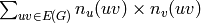
EXAMPLE:
True for any connected graph [1]:
sage: g=graphs.PetersenGraph()
sage: g.wiener_index()<= g.szeged_index()
True
True for all trees [1]:
sage: g=Graph()
sage: g.add_edges(graphs.CubeGraph(5).min_spanning_tree())
sage: g.wiener_index() == g.szeged_index()
True
REFERENCE:
[1] Klavzar S., Rajapakse A., Gutman I. (1996). The Szeged and the Wiener index of graphs. Applied Mathematics Letters, 9 (5), pp. 45-49.
Returns the tensor product, also called the categorical product, of self and other.
The tensor product of and is the graph with vertex set
equal to the Cartesian product of the vertices and , and
is an edge iff - is an edge of self, and -
is an edge of other.
EXAMPLES:
sage: Z = graphs.CompleteGraph(2)
sage: C = graphs.CycleGraph(5)
sage: T = C.tensor_product(Z); T
Graph on 10 vertices
sage: T.plot() # long time
sage: D = graphs.DodecahedralGraph()
sage: P = graphs.PetersenGraph()
sage: T = D.tensor_product(P); T
Graph on 200 vertices
sage: T.plot() # long time
Returns a simple version of itself (i.e., undirected and loops and multiple edges are removed).
EXAMPLES:
sage: G = DiGraph(loops=True,multiedges=True,sparse=True)
sage: G.add_edges( [ (0,0), (1,1), (2,2), (2,3,1), (2,3,2), (3,2) ] )
sage: G.edges(labels=False)
[(0, 0), (1, 1), (2, 2), (2, 3), (2, 3), (3, 2)]
sage: H=G.to_simple()
sage: H.edges(labels=False)
[(2, 3)]
sage: H.is_directed()
False
sage: H.allows_loops()
False
sage: H.allows_multiple_edges()
False
A helper function for finding the genus of a graph. Given a graph and a combinatorial embedding (rot_sys), this function will compute the faces (returned as a list of lists of edges (tuples) of the particular embedding.
Note - rot_sys is an ordered list based on the hash order of the vertices of graph. To avoid confusion, it might be best to set the rot_sys based on a ‘nice_copy’ of the graph.
INPUT:
EXAMPLES:
sage: T = graphs.TetrahedralGraph()
sage: T.trace_faces({0: [1, 3, 2], 1: [0, 2, 3], 2: [0, 3, 1], 3: [0, 1, 2]})
[[(0, 1), (1, 2), (2, 0)],
[(3, 2), (2, 1), (1, 3)],
[(2, 3), (3, 0), (0, 2)],
[(0, 3), (3, 1), (1, 0)]]
Computes the transitive closure of a graph and returns it. The original graph is not modified.
The transitive closure of a graph G has an edge (x,y) if and only if there is a path between x and y in G.
The transitive closure of any strongly connected component of a graph is a complete graph. In particular, the transitive closure of a connected undirected graph is a complete graph. The transitive closure of a directed acyclic graph is a directed acyclic graph representing the full partial order.
EXAMPLES:
sage: g=graphs.PathGraph(4)
sage: g.transitive_closure()
Transitive closure of Path Graph: Graph on 4 vertices
sage: g.transitive_closure()==graphs.CompleteGraph(4)
True
sage: g=DiGraph({0:[1,2], 1:[3], 2:[4,5]})
sage: g.transitive_closure().edges(labels=False)
[(0, 1), (0, 2), (0, 3), (0, 4), (0, 5), (1, 3), (2, 4), (2, 5)]
Returns a transitive reduction of a graph. The original graph is not modified.
A transitive reduction H of G has a path from x to y if and only if there was a path from x to y in G. Deleting any edge of H destroys this property. A transitive reduction is not unique in general. A transitive reduction has the same transitive closure as the original graph.
A transitive reduction of a complete graph is a tree. A transitive reduction of a tree is itself.
EXAMPLES:
sage: g=graphs.PathGraph(4)
sage: g.transitive_reduction()==g
True
sage: g=graphs.CompleteGraph(5)
sage: edges = g.transitive_reduction().edges(); len(edges)
4
sage: g=DiGraph({0:[1,2], 1:[2,3,4,5], 2:[4,5]})
sage: g.transitive_reduction().size()
5
Solves the traveling salesman problem (TSP)
Given a graph (resp. a digraph) with weighted edges,
the traveling salesman problem consists in finding a
hamiltonian cycle (resp. circuit) of the graph of
minimum cost.
This TSP is one of the most famous NP-Complete problems, this function can thus be expected to take some time before returning its result.
INPUT:
weighted (boolean) – whether to consider the weights of the edges.
- If set to False (default), all edges are assumed to weight
- If set to True, the weights are taken into account, and the edges whose weight is None are assumed to be set to
OUTPUT:
A solution to the TSP, as a Graph object whose vertex
set is , and whose edges are only those of the
solution.
ALGORITHM:
This optimization problem is solved through the use of Linear Programming.
NOTE:
EXAMPLES:
The Heawood graph is known to be hamiltonian:
sage: g = graphs.HeawoodGraph()
sage: tsp = g.traveling_salesman_problem()
sage: tsp
TSP from Heawood graph: Graph on 14 vertices
The solution to the TSP has to be connected
sage: tsp.is_connected()
True
It must also be a -regular graph:
sage: tsp.is_regular(k=2)
True
And obviously it is a subgraph of the Heawood graph:
sage: all([ e in g.edges() for e in tsp.edges()])
True
On the other hand, the Petersen Graph is known not to be hamiltonian:
sage: g = graphs.PetersenGraph()
sage: tsp = g.traveling_salesman_problem()
...
ValueError: The given graph is not hamiltonian
One easy way to change is is obviously to add to this graph the edges corresponding to a hamiltonian cycle.
If we do this by setting the cost of these new edges
to , while the others are set to , we notice
that not all the edges we added are used in the
optimal solution
sage: for u, v in g.edges(labels = None):
... g.set_edge_label(u,v,1)
sage: cycle = graphs.CycleGraph(10)
sage: for u,v in cycle.edges(labels = None):
... if not g.has_edge(u,v):
... g.add_edge(u,v)
... g.set_edge_label(u,v,2)
sage: tsp = g.traveling_salesman_problem(weighted = True)
sage: sum( tsp.edge_labels() ) < 2*10
True
If we pick  instead of as a cost for these new edges,
they clearly become the optimal solution
instead of as a cost for these new edges,
they clearly become the optimal solution
sage: for u,v in cycle.edges(labels = None): ... g.set_edge_label(u,v,1/2)
sage: tsp = g.traveling_salesman_problem(weighted = True) sage: sum( tsp.edge_labels() ) == (1/2)*10 True
Returns the union of self and other.
If the graphs have common vertices, the common vertices will be identified.
EXAMPLES:
sage: G = graphs.CycleGraph(3)
sage: H = graphs.CycleGraph(4)
sage: J = G.union(H); J
Graph on 4 vertices
sage: J.vertices()
[0, 1, 2, 3]
sage: J.edges(labels=False)
[(0, 1), (0, 2), (0, 3), (1, 2), (2, 3)]
Returns a list of all vertices in the external boundary of vertices1, intersected with vertices2. If vertices2 is None, then vertices2 is the complement of vertices1. This is much faster if vertices1 is smaller than vertices2.
The external boundary of a set of vertices is the union of the
neighborhoods of each vertex in the set. Note that in this
implementation, since vertices2 defaults to the complement of
vertices1, if a vertex has a loop, then
vertex_boundary(v) will not contain .
In a digraph, the external boundary of a vertex v are those vertices u with an arc (v, u).
EXAMPLES:
sage: G = graphs.CubeGraph(4)
sage: l = ['0111', '0000', '0001', '0011', '0010', '0101', '0100', '1111', '1101', '1011', '1001']
sage: G.vertex_boundary(['0000', '1111'], l)
['0111', '0001', '0010', '0100', '1101', '1011']
sage: D = DiGraph({0:[1,2], 3:[0]})
sage: D.vertex_boundary([0])
[1, 2]
Returns the vertex connectivity of the graph. For more information, see the Wikipedia article on connectivity.
INPUT:
EXAMPLES:
A basic application on a PappusGraph:
sage: g=graphs.PappusGraph()
sage: g.vertex_connectivity()
3.0
In a grid, the vertex connectivity is equal to the
minimum degree, in which case one of the two sets it
of cardinality :
sage: g = graphs.GridGraph([ 3,3 ])
sage: [value, cut, [ setA, setB ]] = g.vertex_connectivity(sets=True)
sage: len(setA) == 1 or len(setB) == 1
True
A vertex cut in a tree is any internal vertex:
sage: g = graphs.RandomGNP(15,.5)
sage: tree = Graph()
sage: tree.add_edges(g.min_spanning_tree())
sage: [val, [cut_vertex]] = tree.vertex_connectivity(value_only=False)
sage: tree.degree(cut_vertex) > 1
True
When value_only = True, this function is optimized for small connexity values and does not need to build a linear program.
It is the case for connected graphs which are not connected:
sage: g = 2 * graphs.PetersenGraph()
sage: g.vertex_connectivity()
0.0
Or if they are just 1-connected:
sage: g = graphs.PathGraph(10)
sage: g.vertex_connectivity()
1.0
For directed graphs, the strong connexity is tested through the dedicated function:
sage: g = digraphs.ButterflyGraph(3)
sage: g.vertex_connectivity()
0.0
Returns a minimum vertex cover of self represented by a list of vertices.
A minimum vertex cover of a graph is a set of
vertices such that each edge is incident to at least
one element of , and such that is of minimum
cardinality. For more information, see the
Wikipedia article on vertex cover.
Equivalently, a vertex cover is defined as the complement of an independent set.
As an optimization problem, it can be expressed as follows:
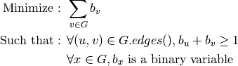
INPUT:
 -complete, its solving
may take some time depending on the graph. A value of 0 means
that there will be no message printed by the solver. This option
is only useful if algorithm="MILP".
-complete, its solving
may take some time depending on the graph. A value of 0 means
that there will be no message printed by the solver. This option
is only useful if algorithm="MILP".EXAMPLES:
On the Pappus graph:
sage: g = graphs.PappusGraph()
sage: g.vertex_cover(value_only=True)
9
The two algorithms should return the same result:
sage: g = graphs.RandomGNP(10,.5)
sage: vc1 = g.vertex_cover(algorithm="MILP")
sage: vc2 = g.vertex_cover(algorithm="Cliquer")
sage: len(vc1) == len(vc2)
True
Returns a minimum vertex cut between non adjacent vertices and
represented by a list of vertices.
A vertex cut between two non adjacent vertices is a set  of vertices of self such that the graph obtained by removing
from self is disconnected. For more information, see the
Wikipedia article on cuts.
of vertices of self such that the graph obtained by removing
from self is disconnected. For more information, see the
Wikipedia article on cuts.
INPUT:
OUTPUT:
Real number or tuple, depending on the given arguments (examples are given below).
EXAMPLE:
A basic application in the Pappus graph:
sage: g = graphs.PappusGraph()
sage: g.vertex_cut(1, 16, value_only=True)
3.0
In the bipartite complete graph  , a cut between the two
vertices in the size part consists of the other vertices:
, a cut between the two
vertices in the size part consists of the other vertices:
sage: g = graphs.CompleteBipartiteGraph(2, 8)
sage: [value, vertices] = g.vertex_cut(0, 1, value_only=False)
sage: print value
8.0
sage: vertices == range(2,10)
True
Clearly, in this case the two sides of the cut are singletons
sage: [value, vertices, [set1, set2]] = g.vertex_cut(0,1, vertices=True)
sage: len(set1) == 1
True
sage: len(set2) == 1
True
Returns a list of vertex-disjoint paths between two vertices as given by Menger’s theorem.
The vertex version of Menger’s theorem asserts that the size
of the minimum vertex cut between two vertices and`t`
(the minimum number of vertices whose removal disconnects
and ) is equal to the maximum number of pairwise
vertex-independent paths from to .
This function returns a list of such paths.
EXAMPLE:
In a complete bipartite graph
sage: g = graphs.CompleteBipartiteGraph(2,3)
sage: g.vertex_disjoint_paths(0,1)
[[0, 2, 1], [0, 3, 1], [0, 4, 1]]
Returns an iterator over the given vertices. Returns False if not given a vertex, sequence, iterator or None. None is equivalent to a list of every vertex. Note that for v in G syntax is allowed.
INPUT:
EXAMPLES:
sage: P = graphs.PetersenGraph()
sage: for v in P.vertex_iterator():
... print v
...
0
1
2
...
8
9
sage: G = graphs.TetrahedralGraph()
sage: for i in G:
... print i
0
1
2
3
Note that since the intersection option is available, the vertex_iterator() function is sub-optimal, speed-wise, but note the following optimization:
sage: timeit V = P.vertices() # not tested
100000 loops, best of 3: 8.85 [micro]s per loop
sage: timeit V = list(P.vertex_iterator()) # not tested
100000 loops, best of 3: 5.74 [micro]s per loop
sage: timeit V = list(P._nxg.adj.iterkeys()) # not tested
100000 loops, best of 3: 3.45 [micro]s per loop
In other words, if you want a fast vertex iterator, call the dictionary directly.
Return a list of the vertices.
INPUT:
EXAMPLES:
sage: P = graphs.PetersenGraph()
sage: P.vertices()
[0, 1, 2, 3, 4, 5, 6, 7, 8, 9]
Note that the output of the vertices() function is always sorted. This is sub-optimal, speed-wise, but note the following optimizations:
sage: timeit V = P.vertices() # not tested
100000 loops, best of 3: 8.85 [micro]s per loop
sage: timeit V = list(P.vertex_iterator()) # not tested
100000 loops, best of 3: 5.74 [micro]s per loop
sage: timeit V = list(P._nxg.adj.iterkeys()) # not tested
100000 loops, best of 3: 3.45 [micro]s per loop
In other words, if you want a fast vertex iterator, call the dictionary directly.
Returns whether the (di)graph is to be considered as a weighted (di)graph.
Note that edge weightings can still exist for (di)graphs G where G.weighted() is False.
EXAMPLES: Here we have two graphs with different labels, but weighted is False for both, so we just check for the presence of edges:
sage: G = Graph({0:{1:'a'}},sparse=True)
sage: H = Graph({0:{1:'b'}},sparse=True)
sage: G == H
True
Now one is weighted and the other is not, and thus the graphs are not equal:
sage: G.weighted(True)
sage: H.weighted()
False
sage: G == H
False
However, if both are weighted, then we finally compare ‘a’ to ‘b’.
sage: H.weighted(True)
sage: G == H
False
Returns the weighted adjacency matrix of the graph. Each vertex is represented by its position in the list returned by the vertices() function.
EXAMPLES:
sage: G = Graph(sparse=True, weighted=True)
sage: G.add_edges([(0,1,1),(1,2,2),(0,2,3),(0,3,4)])
sage: M = G.weighted_adjacency_matrix(); M
[0 1 3 4]
[1 0 2 0]
[3 2 0 0]
[4 0 0 0]
sage: H = Graph(data=M, format='weighted_adjacency_matrix', sparse=True)
sage: H == G
True
The following doctest verifies that #4888 is fixed:
sage: G = DiGraph({0:{}, 1:{0:1}, 2:{0:1}}, weighted = True,sparse=True)
sage: G.weighted_adjacency_matrix()
[0 0 0]
[1 0 0]
[1 0 0]
Returns the Wiener index of the graph.
The Wiener index of a graph can be defined in two equivalent
ways [1] :
 where denotes the distance between
vertices and .
where denotes the distance between
vertices and . be a set of
  paths in such that
contains exactly one shortest
paths in such that
contains exactly one shortest  path for each set
  of vertices
in . Besides,
of vertices
in . Besides,  , let
, let  denote the paths from
containing . We then have
denote the paths from
containing . We then have  .
.EXAMPLE:
From [2], cited in [1]:
sage: g=graphs.PathGraph(10)
sage: w=lambda x: (x*(x*x -1)/6)
sage: g.wiener_index()==w(10)
True
REFERENCE:
[1] Klavzar S., Rajapakse A., Gutman I. (1996). The Szeged and the Wiener index of graphs. Applied Mathematics Letters, 9 (5), pp. 45-49.
[2] I Gutman, YN Yeh, SL Lee, YL Luo (1993), Some recent results in the theory of the Wiener number. INDIAN JOURNAL OF CHEMISTRY SECTION A PUBLICATIONS & INFORMATION DIRECTORATE, CSIR
Helper function for canonical labeling of edge labeled (di)graphs.
Translates to a bipartite incidence-structure type graph appropriate for computing canonical labels of edge labeled graphs. Note that this is actually computationally equivalent to implementing a change on an inner loop of the main algorithm- namely making the refinement procedure sort for each label.
If the graph is a multigraph, it is translated to a non-multigraph, where each edge is labeled with a dictionary describing how many edges of each label were originally there. Then in either case we are working on a graph without multiple edges. At this point, we create another (bipartite) graph, whose left vertices are the original vertices of the graph, and whose right vertices represent the edges. We partition the left vertices as they were originally, and the right vertices by common labels: only automorphisms taking edges to like-labeled edges are allowed, and this additional partition information enforces this on the bipartite graph.
EXAMPLES:
sage: G = Graph(multiedges=True,sparse=True)
sage: G.add_edges([(0,1,i) for i in range(10)])
sage: G.add_edge(1,2,'string')
sage: G.add_edge(2,3)
sage: from sage.graphs.generic_graph import graph_isom_equivalent_non_edge_labeled_graph
sage: graph_isom_equivalent_non_edge_labeled_graph(G, [G.vertices()])
(Graph on 7 vertices, [[('o', 0), ('o', 1), ('o', 2), ('o', 3)], [('x', 2)], [('x', 0)], [('x', 1)]])
Helper function for canonical labeling of multi-(di)graphs.
The idea for this function is that the main algorithm for computing
isomorphism of graphs does not allow multiple edges. Instead of
making some very difficult changes to that, we can simply modify
the multigraph into a non-multi graph that carries essentially the
same information. For each pair of vertices , if
there is at most one edge between and , we
do nothing, but if there are more than one, we split each edge into
two, introducing a new vertex. These vertices really represent
edges, so we keep them in their own part of a partition - to
distinguish them from genuine vertices. Then the canonical label
and automorphism group is computed, and in the end, we strip off
the parts of the generators that describe how these new vertices
move, and we have the automorphism group of the original
multi-graph. Similarly, by putting the additional vertices in their
own cell of the partition, we guarantee that the relabeling leading
to a canonical label moves genuine vertices amongst themselves, and
hence the canonical label is still well-defined, when we forget
about the additional vertices.
EXAMPLES:
sage: from sage.graphs.generic_graph import graph_isom_equivalent_non_multi_graph
sage: G = Graph(multiedges=True,sparse=True)
sage: G.add_edge((0,1,1))
sage: G.add_edge((0,1,2))
sage: G.add_edge((0,1,3))
sage: graph_isom_equivalent_non_multi_graph(G, [[0,1]])
(Graph on 5 vertices, [[('o', 0), ('o', 1)], [('x', 0), ('x', 1), ('x', 2)]])
Helper function for plotting graphs in 3d with Tachyon. Returns a plot containing only the vertices, as well as the 3d position dictionary used for the plot.
 - a 3D layout of the vertices
EXAMPLES:
sage: G = graphs.TetrahedralGraph()
sage: from sage.graphs.generic_graph import tachyon_vertex_plot
sage: T,p = tachyon_vertex_plot(G, pos3d = G.layout(dim=3))
sage: type(T)
<class 'sage.plot.plot3d.tachyon.Tachyon'>
sage: type(p)
<type 'dict'>