Partitions¶

A partition $p$ of a nonnegative integer $n$ is a non-increasing list of positive integers (the parts of the partition) with total sum $n$ .

A partition can be depicted by a diagram made of rows of cells, where the number of cells in the $i^{th}$ row starting from the top is the $i^{th}$ part of the partition.

The coordinate system related to a partition applies from the top to the bottom and from left to right. So, the corners of the partition are [[0,4], [1,2], [2,0]].

AUTHORS:

Mike Hansen (2007): initial version
Dan Drake (2009-03-28): deprecate RestrictedPartitions and implement Partitions_parts_in

EXAMPLES:

There are 5 partitions of the integer 4:

sage: Partitions(4).cardinality()
5
sage: Partitions(4).list()
[[4], [3, 1], [2, 2], [2, 1, 1], [1, 1, 1, 1]]

We can use the method .first() to get the ‘first’ partition of a number:

sage: Partitions(4).first()
[4]

Using the method .next(), we can calculate the ‘next’ partition. When we are at the last partition, None will be returned:

sage: Partitions(4).next([4])
[3, 1]
sage: Partitions(4).next([1,1,1,1]) is None
True

We can use iter to get an object which iterates over the partitions one by one to save memory. Note that when we do something like for part in Partitions(4) this iterator is used in the background:

sage: g = iter(Partitions(4))

sage: g.next()
[4]
sage: g.next()
[3, 1]
sage: g.next()
[2, 2]
sage: for p in Partitions(4): print p
[4]
[3, 1]
[2, 2]
[2, 1, 1]
[1, 1, 1, 1]

We can add constraints to to the type of partitions we want. For example, to get all of the partitions of 4 of length 2, we’d do the following:

sage: Partitions(4, length=2).list()
[[3, 1], [2, 2]]

Here is the list of partitions of length at least 2 and the list of ones with length at most 2:

sage: Partitions(4, min_length=2).list()
[[3, 1], [2, 2], [2, 1, 1], [1, 1, 1, 1]]
sage: Partitions(4, max_length=2).list()
[[4], [3, 1], [2, 2]]

The options min_part and max_part can be used to set constraints on the sizes of all parts. Using max_part, we can select partitions having only ‘small’ entries. The following is the list of the partitions of 4 with parts at most 2:

sage: Partitions(4, max_part=2).list()
[[2, 2], [2, 1, 1], [1, 1, 1, 1]]

The min_part options is complementary to max_part and selects partitions having only ‘large’ parts. Here is the list of all partitions of 4 with each part at least 2:

sage: Partitions(4, min_part=2).list()
[[4], [2, 2]]

The options inner and outer can be used to set part-by-part constraints. This is the list of partitions of 4 with [3, 1, 1] as an outer bound:

sage: Partitions(4, outer=[3,1,1]).list()
[[3, 1], [2, 1, 1]]

Outer sets max_length to the length of its argument. Moreover, the parts of outer may be infinite to clear constraints on specific parts. Here is the list of the partitions of 4 of length at most 3 such that the second and third part are 1 when they exist:

sage: Partitions(4, outer=[oo,1,1]).list()
[[4], [3, 1], [2, 1, 1]]

Finally, here are the partitions of 4 with [1,1,1] as an inner bound. Note that inner sets min_length to the length of its argument:

sage: Partitions(4, inner=[1,1,1]).list()
[[2, 1, 1], [1, 1, 1, 1]]

The options min_slope and max_slope can be used to set constraints on the slope, that is on the difference p[i+1]-p[i] of two consecutive parts. Here is the list of the strictly decreasing partitions of 4:

sage: Partitions(4, max_slope=-1).list()
[[4], [3, 1]]

The constraints can be combined together in all reasonable ways. Here are all the partitions of 11 of length between 2 and 4 such that the difference between two consecutive parts is between -3 and -1:

sage: Partitions(11,min_slope=-3,max_slope=-1,min_length=2,max_length=4).list()
[[7, 4], [6, 5], [6, 4, 1], [6, 3, 2], [5, 4, 2], [5, 3, 2, 1]]

Partition objects can also be created individually with the Partition function:

sage: Partition([2,1])
[2, 1]

Once we have a partition object, then there are a variety of methods that we can use. For example, we can get the conjugate of a partition. Geometrically, the conjugate of a partition is the reflection of that partition through its main diagonal. Of course, this operation is an involution:

sage: Partition([4,1]).conjugate()
[2, 1, 1, 1]
sage: Partition([4,1]).conjugate().conjugate()
[4, 1]

We can go back and forth between the exponential notations of a partition. The exponential notation can be padded with extra zeros:

sage: Partition([6,4,4,2,1]).to_exp()
[1, 1, 0, 2, 0, 1]
sage: Partition(exp=[1,1,0,2,0,1])
[6, 4, 4, 2, 1]
sage: Partition([6,4,4,2,1]).to_exp(5)
[1, 1, 0, 2, 0, 1]
sage: Partition([6,4,4,2,1]).to_exp(7)
[1, 1, 0, 2, 0, 1, 0]
sage: Partition([6,4,4,2,1]).to_exp(10)
[1, 1, 0, 2, 0, 1, 0, 0, 0, 0]

We can get the coordinates of the corners of a partition:

sage: Partition([4,3,1]).corners()
[(0, 3), (1, 2), (2, 0)]

We can compute the core and quotient of a partition and build the partition back up from them:

sage: Partition([6,3,2,2]).core(3)
[2, 1, 1]
sage: Partition([7,7,5,3,3,3,1]).quotient(3)
[[2], [1], [2, 2, 2]]
sage: p = Partition([11,5,5,3,2,2,2])
sage: p.core(3)
[]
sage: p.quotient(3)
[[2, 1], [4], [1, 1, 1]]
sage: Partition(core=[],quotient=[[2, 1], [4], [1, 1, 1]])
[11, 5, 5, 3, 2, 2, 2]

sage.combinat.partition.OrderedPartitions(n, k=None)¶

Returns the combinatorial class of ordered partitions of n. If k is specified, then only the ordered partitions of length k are returned.

Note

It is recommended that you use Compositions instead as OrderedPartitions wraps GAP. See also ordered_partitions.

EXAMPLES:

sage: OrderedPartitions(3)
Ordered partitions of 3
sage: OrderedPartitions(3).list()
[[3], [2, 1], [1, 2], [1, 1, 1]]
sage: OrderedPartitions(3,2)
Ordered partitions of 3 of length 2
sage: OrderedPartitions(3,2).list()
[[2, 1], [1, 2]]

class sage.combinat.partition.OrderedPartitions_nk(n, k=None)¶

Bases: sage.combinat.combinat.CombinatorialClass

cardinality()¶

EXAMPLES:

sage: OrderedPartitions(3).cardinality()
4
sage: OrderedPartitions(3,2).cardinality()
2

list()¶

EXAMPLES:

sage: OrderedPartitions(3).list()
[[3], [2, 1], [1, 2], [1, 1, 1]]
sage: OrderedPartitions(3,2).list()
[[2, 1], [1, 2]]

sage.combinat.partition.Partition(mu=None, **keyword)¶

A partition is a weakly decreasing ordered sequence of non-negative integers. This function returns a Sage partition object which can be specified in one of the following ways:

* a list (the default)
* using exponential notation
* by beta numbers (TODO)
* specifying the core and the quotient
* specifying the core and the canonical quotient (TODO)

See the examples below.

Sage follows the usual python conventions when dealing with partitions, so that the first part of the partition mu=Partition([4,3,2,2]) is mu[0], the second part is mu[1] and so on. As is usual, Sage ignores trailing zeros at the end of partitions.

EXAMPLES:

sage: Partition([3,2,1])
[3, 2, 1]
sage: Partition([3,2,1,0])
[3, 2, 1]
sage: Partition(exp=[2,1,1])
[3, 2, 1, 1]
sage: Partition(core=[2,1], quotient=[[2,1],[3],[1,1,1]])
[11, 5, 5, 3, 2, 2, 2]
sage: [2,1] in Partitions()
True
sage: [2,1,0] in Partitions()
False
sage: Partition([1,2,3])
...
ValueError: [1, 2, 3] is not a valid partition

sage.combinat.partition.PartitionTuples(n, k)¶

Returns the combinatorial class of k-tuples of partitions of n. These are are ordered list of k partitions whose sizes add up to

TODO: reimplement in term of species.ProductSpecies and Partitions

These describe the classes and the characters of wreath products of groups with k conjugacy classes with the symmetric group $S_n$ .

EXAMPLES:

sage: PartitionTuples(4,2)
2-tuples of partitions of 4
sage: PartitionTuples(3,2).list()
[[[3], []],
 [[2, 1], []],
 [[1, 1, 1], []],
 [[2], [1]],
 [[1, 1], [1]],
 [[1], [2]],
 [[1], [1, 1]],
 [[], [3]],
 [[], [2, 1]],
 [[], [1, 1, 1]]]

class sage.combinat.partition.PartitionTuples_nk(n, k)¶

Bases: sage.combinat.combinat.CombinatorialClass

Element¶: alias of Partition_class

cardinality()¶

Returns the number of k-tuples of partitions which together form a partition of n.

Wraps GAP’s NrPartitionTuples.

EXAMPLES:

sage: PartitionTuples(3,2).cardinality()
10
sage: PartitionTuples(8,2).cardinality()
185

Now we compare that with the result of the following GAP computation:

gap> S8:=Group((1,2,3,4,5,6,7,8),(1,2));
Group([ (1,2,3,4,5,6,7,8), (1,2) ])
gap> C2:=Group((1,2));
Group([ (1,2) ])
gap> W:=WreathProduct(C2,S8);
<permutation group of size 10321920 with 10 generators>
gap> Size(W);
10321920     ## = 2^8*Factorial(8), which is good:-)
gap> Size(ConjugacyClasses(W));
185

class sage.combinat.partition.Partition_class(l)¶

Bases: sage.combinat.combinat.CombinatorialObject

add_box(*args, **kwds)¶

Returns a partition corresponding to self with a cell added in row i. i and j are 0-based row and column indices. This does not change p.

Note that if you have coordinates in a list, you can call this function with python’s * notation (see the examples below).

EXAMPLES:

sage: Partition([3, 2, 1, 1]).add_cell(0)
[4, 2, 1, 1]
sage: cell = [4, 0]; Partition([3, 2, 1, 1]).add_cell(*cell)
[3, 2, 1, 1, 1]

add_cell(i, j=None)¶

Returns a partition corresponding to self with a cell added in row i. i and j are 0-based row and column indices. This does not change p.

Note that if you have coordinates in a list, you can call this function with python’s * notation (see the examples below).

EXAMPLES:

sage: Partition([3, 2, 1, 1]).add_cell(0)
[4, 2, 1, 1]
sage: cell = [4, 0]; Partition([3, 2, 1, 1]).add_cell(*cell)
[3, 2, 1, 1, 1]

add_horizontal_border_strip(k)¶

Returns a list of all the partitions that can be obtained by adding a horizontal border strip of length k to self.

EXAMPLES:

sage: Partition([]).add_horizontal_border_strip(0)
[[]]
sage: Partition([]).add_horizontal_border_strip(2)
[[2]]
sage: Partition([2,2]).add_horizontal_border_strip(2)
[[2, 2, 2], [3, 2, 1], [4, 2]]
sage: Partition([3,2,2]).add_horizontal_border_strip(2)
[[3, 2, 2, 2], [3, 3, 2, 1], [4, 2, 2, 1], [4, 3, 2], [5, 2, 2]]

TODO: reimplement like remove_horizontal_border_strip using IntegerListsLex

add_vertical_border_strip(k)¶

Returns a list of all the partitions that can be obtained by adding a vertical border strip of length k to self.

EXAMPLES:

sage: Partition([]).add_vertical_border_strip(0)
[[]]
sage: Partition([]).add_vertical_border_strip(2)
[[1, 1]]
sage: Partition([2,2]).add_vertical_border_strip(2)
[[3, 3], [3, 2, 1], [2, 2, 1, 1]]
sage: Partition([3,2,2]).add_vertical_border_strip(2)
[[4, 3, 2], [4, 2, 2, 1], [3, 3, 3], [3, 3, 2, 1], [3, 2, 2, 1, 1]]

arm(*args, **kwds)¶

Returns the length of the arm of cell (i,j) in partition p.

INPUT: i and j: two integers

OUPUT: an integer or a ValueError

The arm of cell (i,j) is the cells that appear to the right of cell (i,j). Note that i and j are 0-based indices. If your coordinates are in the form (i,j), use Python’s *-operator.

EXAMPLES:

sage: p = Partition([2,2,1])
sage: p.arm_length(0, 0)
1
sage: p.arm_length(0, 1)
0
sage: p.arm_length(2, 0)
0
sage: Partition([3,3]).arm_length(0, 0)
2
sage: Partition([3,3]).arm_length(*[0,0])
2

arm_cells(i, j)¶

Returns the list of the cells of the arm of cell (i,j) in partition p.

INPUT: i and j: two integers

OUTPUT: a list of pairs of integers

The arm of cell (i,j) is the boxes that appear to the right of cell (i,j). Note that i and j are 0-based indices. If your coordinates are in the form (i,j), use Python’s *-operator.

Examples:

sage: Partition([4,4,3,1]).arm_cells(1,1)
[(1, 2), (1, 3)]

sage: Partition([]).arm_cells(0,0)
...
ValueError: The cells is not in the diagram

arm_length(i, j)¶

Returns the length of the arm of cell (i,j) in partition p.

INPUT: i and j: two integers

OUPUT: an integer or a ValueError

The arm of cell (i,j) is the cells that appear to the right of cell (i,j). Note that i and j are 0-based indices. If your coordinates are in the form (i,j), use Python’s *-operator.

EXAMPLES:

sage: p = Partition([2,2,1])
sage: p.arm_length(0, 0)
1
sage: p.arm_length(0, 1)
0
sage: p.arm_length(2, 0)
0
sage: Partition([3,3]).arm_length(0, 0)
2
sage: Partition([3,3]).arm_length(*[0,0])
2

arm_lengths(flat=False)¶

Returns a tableau of shape p where each cell is filled its arm length. The optional boolean parameter flat provides the option of returning a flat list.

EXAMPLES:

sage: Partition([2,2,1]).arm_lengths()
[[1, 0], [1, 0], [0]]
sage: Partition([2,2,1]).arm_lengths(flat=True)
[1, 0, 1, 0, 0]
sage: Partition([3,3]).arm_lengths()
[[2, 1, 0], [2, 1, 0]]
sage: Partition([3,3]).arm_lengths(flat=True)
[2, 1, 0, 2, 1, 0]

arms_legs_coeff(i, j)¶

This is a statistic on a cell c=(i,j) in the diagram of partition p given by

$[ (1 - q^{arm_length(c)} * t^{leg_length(c) + 1}) ] / [ (1 - q^{arm_length(c) + 1} * t^{leg_length(c)}) ]$

EXAMPLES:

sage: Partition([3,2,1]).arms_legs_coeff(1,1)
(-t + 1)/(-q + 1)
sage: Partition([3,2,1]).arms_legs_coeff(0,0)
(-q^2*t^3 + 1)/(-q^3*t^2 + 1)
sage: Partition([3,2,1]).arms_legs_coeff(*[0,0])
(-q^2*t^3 + 1)/(-q^3*t^2 + 1)

associated(*args, **kwds)¶

Returns the conjugate partition of the partition self. This is also called the associated partition in the literature.

EXAMPLES:

sage: Partition([2,2]).conjugate()
[2, 2]
sage: Partition([6,3,1]).conjugate()
[3, 2, 2, 1, 1, 1]

The conjugate partition is obtained by transposing the Ferrers diagram of the partition (see ferrers_diagram()):

sage: print Partition([6,3,1]).ferrers_diagram()
******
***
*
sage: print Partition([6,3,1]).conjugate().ferrers_diagram()
***
**
**
*
*
*

atom()¶

Returns a list of the standard tableaux of size self.size() whose atom is equal to self.

EXAMPLES:

sage: Partition([2,1]).atom()
[[[1, 2], [3]]]
sage: Partition([3,2,1]).atom()
[[[1, 2, 3, 6], [4, 5]], [[1, 2, 3], [4, 5], [6]]]

aut()¶

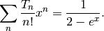
Returns a factor for the number of permutations with cycle type self. self.aut() returns $1^{j_1}j_1! \cdots n^{j_n}j_n!$ where $j_k$ is the number of parts in self equal to k.

The number of permutations having $p$ as a cycle type is given by

$\frac{n!}{1^{j_1}j_1! \cdots n^{j_n}j_n!} .$

EXAMPLES:

sage: Partition([2,1]).aut()
2

boxes(*args, **kwds)¶

Return the coordinates of the cells of self. Coordinates are given as (row-index, column-index) and are 0 based.

EXAMPLES:

sage: Partition([2,2]).cells()
[(0, 0), (0, 1), (1, 0), (1, 1)]
sage: Partition([3,2]).cells()
[(0, 0), (0, 1), (0, 2), (1, 0), (1, 1)]

cells()¶

Return the coordinates of the cells of self. Coordinates are given as (row-index, column-index) and are 0 based.

EXAMPLES:

sage: Partition([2,2]).cells()
[(0, 0), (0, 1), (1, 0), (1, 1)]
sage: Partition([3,2]).cells()
[(0, 0), (0, 1), (0, 2), (1, 0), (1, 1)]

centralizer_size(t=0, q=0)¶

Returns the size of the centralizer of any permutation of cycle type self. If m_i is the multiplicity of i as a part of p, this is given by $\prod_i (i^m[i])*(m[i]!)$ . Including the optional parameters t and q gives the q-t analog which is the former product times $\prod_{i=1}^{length(p)} (1 - q^{p[i]}) / (1 - t^{p[i]}).$

EXAMPLES:

sage: Partition([2,2,1]).centralizer_size()
8
sage: Partition([2,2,2]).centralizer_size()
48 

REFERENCES:

Kerber, A. ‘Algebraic Combinatorics via Finite Group Action’, 1.3 p24

character_polynomial()¶

Returns the character polynomial associated to the partition self. The character polynomial $q_\mu$ is defined by

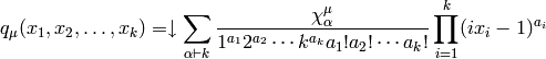
$q_\mu(x_1, x_2, \ldots, x_k) = \downarrow \sum_{\alpha \vdash k}\frac{ \chi^\mu_\alpha }{1^{a_1}2^{a_2}\cdots k^{a_k}a_1!a_2!\cdots a_k!} \prod_{i=1}^{k} (ix_i-1)^{a_i}$

where $a_i$ is the multiplicity of $i$ in $\alpha$ .

It is computed in the following manner.

Expand the Schur function $s_\mu$ in the power-sum basis.
Replace each $p_i$ with $ix_i-1$
Apply the umbral operator $\downarrow$ to the resulting polynomial.

EXAMPLES:

sage: Partition([1]).character_polynomial()
x - 1
sage: Partition([1,1]).character_polynomial()
1/2*x0^2 - 3/2*x0 - x1 + 1
sage: Partition([2,1]).character_polynomial()
1/3*x0^3 - 2*x0^2 + 8/3*x0 - x2

conjugacy_class_size()¶

Returns the size of the conjugacy class of the symmetric group indexed by the partition p.

EXAMPLES:

sage: Partition([2,2,2]).conjugacy_class_size()
15
sage: Partition([2,2,1]).conjugacy_class_size()
15
sage: Partition([2,1,1]).conjugacy_class_size() 
6

REFERENCES:

Kerber, A. ‘Algebraic Combinatorics via Finite Group Action’ 1.3 p24

conjugate()¶

Returns the conjugate partition of the partition self. This is also called the associated partition in the literature.

EXAMPLES:

sage: Partition([2,2]).conjugate()
[2, 2]
sage: Partition([6,3,1]).conjugate()
[3, 2, 2, 1, 1, 1]

The conjugate partition is obtained by transposing the Ferrers diagram of the partition (see ferrers_diagram()):

sage: print Partition([6,3,1]).ferrers_diagram()
******
***
*
sage: print Partition([6,3,1]).conjugate().ferrers_diagram()
***
**
**
*
*
*

contains(x)¶

Returns True if p2 is a partition whose Ferrers diagram is contained in the Ferrers diagram of self

EXAMPLES:

sage: p = Partition([3,2,1])
sage: p.contains([2,1])
True
sage: all(p.contains(mu) for mu in Partitions(3))
True
sage: all(p.contains(mu) for mu in Partitions(4))
False

content(i, j)¶

Returns the content statistic of the given cell, which is simply defined by j - i. This doesn’t technically depend on the partition, but is included here because it is often useful in the context of partitions.

EXAMPLES:

sage: Partition([2,1]).content(0,1)
1
sage: p = Partition([3,2])
sage: sum([p.content(*c) for c in p.cells()])
2

core(length)¶

Returns the core of the partition – in the literature the core is commonly referred to as the $k$ -core, $p$ -core, $r$ -core, ... . The construction of the core can be visualized by repeatedly removing border strips of size $r$ from self until this is no longer possible. The remaining partition is the core.

EXAMPLES:

sage: Partition([6,3,2,2]).core(3)
[2, 1, 1]
sage: Partition([]).core(3)
[]
sage: Partition([8,7,7,4,1,1,1,1,1]).core(3)
[2, 1, 1]

TESTS:

sage: Partition([3,3,3,2,1]).core(3)
[]
sage: Partition([10,8,7,7]).core(4)
[]
sage: Partition([21,15,15,9,6,6,6,3,3]).core(3)
[]

corners()¶

Returns a list of the corners of the partitions. These are the positions where we can remove a cell. Indices are of the form (i,j) where i is the row-index and j is the column-index, and are 0-based.

EXAMPLES:

sage: Partition([3,2,1]).corners()
[(0, 2), (1, 1), (2, 0)]
sage: Partition([3,3,1]).corners()
[(1, 2), (2, 0)]

dominate(rows=None)¶

Returns a list of the partitions dominated by n. If n is specified, then it only returns the ones with = rows rows.

EXAMPLES:

sage: Partition([3,2,1]).dominate()
[[3, 2, 1], [3, 1, 1, 1], [2, 2, 2], [2, 2, 1, 1], [2, 1, 1, 1, 1], [1, 1, 1, 1, 1, 1]]
sage: Partition([3,2,1]).dominate(rows=3)
[[3, 2, 1], [2, 2, 2]]

dominates(p2)¶

Returns True if partition p1 dominates partitions p2. Otherwise, it returns False.

EXAMPLES:

sage: p = Partition([3,2])
sage: p.dominates([3,1])
True
sage: p.dominates([2,2])
True
sage: p.dominates([2,1,1])
True
sage: p.dominates([3,3])
False
sage: p.dominates([4])
False
sage: Partition([4]).dominates(p)
False
sage: Partition([]).dominates([1])
False
sage: Partition([]).dominates([])
True
sage: Partition([1]).dominates([])
True

down()¶

Returns a generator for partitions that can be obtained from p by removing a cell.

EXAMPLES:

sage: [p for p in Partition([2,1,1]).down()]
[[1, 1, 1], [2, 1]]
sage: [p for p in Partition([3,2]).down()]
[[2, 2], [3, 1]]
sage: [p for p in Partition([3,2,1]).down()]
[[2, 2, 1], [3, 1, 1], [3, 2]]

down_list()¶

Returns a list of the partitions that can be obtained from the partition p by removing a cell.

EXAMPLES:

sage: Partition([2,1,1]).down_list()
[[1, 1, 1], [2, 1]]
sage: Partition([3,2]).down_list()
[[2, 2], [3, 1]]
sage: Partition([3,2,1]).down_list()
[[2, 2, 1], [3, 1, 1], [3, 2]]

evaluation()¶

Returns the evaluation of the partition.

EXAMPLES:

sage: Partition([4,3,1,1]).evaluation()
[2, 0, 1, 1]

ferrers_diagram()¶

Return the Ferrers diagram of pi.

INPUT:

pi - a partition, given as a list of integers.

EXAMPLES:

sage: print Partition([5,5,2,1]).ferrers_diagram()
*****
*****
**
*

from_kbounded_to_grassmannian(p, k)¶

Maps a $k$ -bounded partition to a Grassmannian element in the affine Weyl group of type $A_k^{(1)}$ .

For details, see the documentation of the method from_kbounded_to_reduced_word() .

EXAMPLES:

sage: p=Partition([2,1,1])
sage: p.from_kbounded_to_grassmannian(2)
[-1  1  1]
[-2  2  1]
[-2  1  2]
sage: p=Partition([])
sage: p.from_kbounded_to_grassmannian(2)
[1 0 0]
[0 1 0]
[0 0 1]

from_kbounded_to_reduced_word(p, k)¶

Maps a $k$ -bounded partition to a reduced word for an element in the affine permutation group.

This uses the fact that there is a bijection between $k$ -bounded partitions and $(k+1)$ -cores and an action of the affine nilCoxeter algebra of type $A_k^{(1)}$ on $(k+1)$ -cores as described in [LM2006].

REFERENCES:

[LM2006] MR2167475 (2006j:05214) L. Lapointe, J. Morse. Tableaux on $k+1$ -cores, reduced words for affine permutations, and $k$ -Schur expansions. J. Combin. Theory Ser. A 112 (2005), no. 1, 44–81.

EXAMPLES:

sage: p=Partition([2,1,1])
sage: p.from_kbounded_to_reduced_word(2)
[2, 1, 2, 0]
sage: p=Partition([3,1])
sage: p.from_kbounded_to_reduced_word(3)
[3, 2, 1, 0]
sage: p.from_kbounded_to_reduced_word(2)
...
ValueError: the partition must be 2-bounded
sage: p=Partition([])
sage: p.from_kbounded_to_reduced_word(2)
[]

generalized_pochhammer_symbol(a, alpha)¶

Returns the generalized Pochhammer symbol $(a)_{self}^{(\alpha)}$ . This is the product over all cells (i,j) in p of $a - (i-1) / \alpha + j - 1$ .

EXAMPLES:

sage: Partition([2,2]).generalized_pochhammer_symbol(2,1)
12

hook(*args, **kwds)¶

Returns the length of the hook of cell (i,j) in the partition p. The hook of cell (i,j) is defined as the cells to the right or below (in the English convention). Note that i and j are 0-based. If your coordinates are in the form (i,j), use Python’s *-operator.

EXAMPLES:

sage: p = Partition([2,2,1])
sage: p.hook_length(0, 0)
4
sage: p.hook_length(0, 1)
2
sage: p.hook_length(2, 0)
1        
sage: Partition([3,3]).hook_length(0, 0)
4        
sage: cell = [0,0]; Partition([3,3]).hook_length(*cell)
4

hook_length(i, j)¶

Returns the length of the hook of cell (i,j) in the partition p. The hook of cell (i,j) is defined as the cells to the right or below (in the English convention). Note that i and j are 0-based. If your coordinates are in the form (i,j), use Python’s *-operator.

EXAMPLES:

sage: p = Partition([2,2,1])
sage: p.hook_length(0, 0)
4
sage: p.hook_length(0, 1)
2
sage: p.hook_length(2, 0)
1        
sage: Partition([3,3]).hook_length(0, 0)
4        
sage: cell = [0,0]; Partition([3,3]).hook_length(*cell)
4

hook_lengths()¶

Returns a tableau of shape p with the cells filled in with the hook lengths.

In each cell, put the sum of one plus the number of cells horizontally to the right and vertically below the cell (the hook length).

For example, consider the partition [3,2,1] of 6 with Ferrers Diagram:

# # #
# #
#

When we fill in the cells with the hook lengths, we obtain:

5 3 1
3 1
1

EXAMPLES:

sage: Partition([2,2,1]).hook_lengths()
[[4, 2], [3, 1], [1]]
sage: Partition([3,3]).hook_lengths()
[[4, 3, 2], [3, 2, 1]]
sage: Partition([3,2,1]).hook_lengths()
[[5, 3, 1], [3, 1], [1]]
sage: Partition([2,2]).hook_lengths()
[[3, 2], [2, 1]]
sage: Partition([5]).hook_lengths()
[[5, 4, 3, 2, 1]]

REFERENCES:

http://mathworld.wolfram.com/HookLengthFormula.html

hook_polynomial(q, t)¶

Returns the two-variable hook polynomial.

EXAMPLES:

sage: R.<q,t> = PolynomialRing(QQ)
sage: a = Partition([2,2]).hook_polynomial(q,t)
sage: a == (1 - t)*(1 - q*t)*(1 - t^2)*(1 - q*t^2)
True
sage: a = Partition([3,2,1]).hook_polynomial(q,t)
sage: a == (1 - t)^3*(1 - q*t^2)^2*(1 - q^2*t^3)
True

hook_product(a)¶

Returns the Jack hook-product.

EXAMPLES:

sage: Partition([3,2,1]).hook_product(x)
(x + 2)^2*(2*x + 3)
sage: Partition([2,2]).hook_product(x)
2*(x + 1)*(x + 2)

hooks()¶

Returns a sorted list of the hook lengths in self.

EXAMPLES:

sage: Partition([3,2,1]).hooks()
[5, 3, 3, 1, 1, 1]

jacobi_trudi()¶

EXAMPLES:

sage: part = Partition([3,2,1])
sage: jt = part.jacobi_trudi(); jt
[h[3] h[1]    0]
[h[4] h[2]  h[]]
[h[5] h[3] h[1]]
sage: s = SFASchur(QQ)
sage: h = SFAHomogeneous(QQ)
sage: h( s(part) )
h[3, 2, 1] - h[3, 3] - h[4, 1, 1] + h[5, 1]
sage: jt.det()
h[3, 2, 1] - h[3, 3] - h[4, 1, 1] + h[5, 1]

k_atom(k)¶

EXAMPLES:

sage: p = Partition([3,2,1])
sage: p.k_atom(1)
[]
sage: p.k_atom(3)
[[[1, 1, 1], [2, 2], [3]],
 [[1, 1, 1, 2], [2], [3]],
 [[1, 1, 1, 3], [2, 2]],
 [[1, 1, 1, 2, 3], [2]]]
sage: Partition([3,2,1]).k_atom(4)
[[[1, 1, 1], [2, 2], [3]], [[1, 1, 1, 3], [2, 2]]]

TESTS:

sage: Partition([1]).k_atom(1)
[[[1]]]
sage: Partition([1]).k_atom(2)
[[[1]]]
sage: Partition([]).k_atom(1)
[[]]

k_conjugate(k)¶

Returns the k-conjugate of the partition.

The k-conjugate is the partition that is given by the columns of the k-skew diagram of the partition.

EXAMPLES:

sage: p = Partition([4,3,2,2,1,1])
sage: p.k_conjugate(4)
[3, 2, 2, 1, 1, 1, 1, 1, 1]

k_skew(k)¶

Returns the k-skew partition.

The k-skew diagram of a k-bounded partition is the skew diagram denoted $\lambda/^k$ satisfying the conditions:

row i of $\lambda/^k$ has length $\lambda_i$
no cell in $\lambda/^k$ has hook-length exceeding k
every square above the diagram of $\lambda/^k$ has hook length exceeding k.

REFERENCES:

Lapointe, L. and Morse, J. ‘Order Ideals in Weak Subposets of Young’s Lattice and Associated Unimodality Conjectures’

EXAMPLES:

sage: p = Partition([4,3,2,2,1,1])
sage: p.k_skew(4)
[[9, 5, 3, 2, 1, 1], [5, 2, 1]]

k_split(k)¶

Returns the k-split of self.

EXAMPLES:

sage: Partition([4,3,2,1]).k_split(3)
[]
sage: Partition([4,3,2,1]).k_split(4)
[[4], [3, 2], [1]]
sage: Partition([4,3,2,1]).k_split(5)
[[4, 3], [2, 1]]
sage: Partition([4,3,2,1]).k_split(6)
[[4, 3, 2], [1]]
sage: Partition([4,3,2,1]).k_split(7)
[[4, 3, 2, 1]]
sage: Partition([4,3,2,1]).k_split(8)
[[4, 3, 2, 1]]

leg(*args, **kwds)¶

Returns the length of the leg of cell (i,j) in partition p.

INPUT: i and j: two integers

OUPUT: an integer or a ValueError

The leg of cell (i,j) is defined to be the cells below it in partition p (in English convention). Note that i and j are 0-based. If your coordinates are in the form (i,j), use Python’s *-operator.

EXAMPLES:

sage: p = Partition([2,2,1])
sage: p.leg_length(0, 0)
2
sage: p.leg_length(0,1)
1
sage: p.leg_length(2,0)
0
sage: Partition([3,3]).leg_length(0, 0)
1
sage: cell = [0,0]; Partition([3,3]).leg_length(*cell)
1

leg_cells(i, j)¶

Returns the list of the cells of the leg of cell (i,j) in partition p.

INPUT: i and j: two integers

OUTPUT: a list of pairs of integers

The leg of cell (i,j) is defined to be the cells below it in partition p (in English convention). Note that i and j are 0-based. If your coordinates are in the form (i,j), use Python’s *-operator.

Examples:

sage: Partition([4,4,3,1]).leg_cells(1,1)
[(2, 1)]
sage: Partition([4,4,3,1]).leg_cells(0,1)
[(1, 1), (2, 1)]

sage: Partition([]).leg_cells(0,0)
...
ValueError: The cells is not in the diagram

leg_length(i, j)¶

Returns the length of the leg of cell (i,j) in partition p.

INPUT: i and j: two integers

OUPUT: an integer or a ValueError

The leg of cell (i,j) is defined to be the cells below it in partition p (in English convention). Note that i and j are 0-based. If your coordinates are in the form (i,j), use Python’s *-operator.

EXAMPLES:

sage: p = Partition([2,2,1])
sage: p.leg_length(0, 0)
2
sage: p.leg_length(0,1)
1
sage: p.leg_length(2,0)
0
sage: Partition([3,3]).leg_length(0, 0)
1
sage: cell = [0,0]; Partition([3,3]).leg_length(*cell)
1

leg_lengths(flat=False)¶

Returns a tableau of shape p with each cell filled in with its leg length. The optional boolean parameter flat provides the option of returning a flat list.

EXAMPLES:

sage: Partition([2,2,1]).leg_lengths()
[[2, 1], [1, 0], [0]]
sage: Partition([2,2,1]).leg_lengths(flat=True)
[2, 1, 1, 0, 0]
sage: Partition([3,3]).leg_lengths()
[[1, 1, 1], [0, 0, 0]]
sage: Partition([3,3]).leg_lengths(flat=True)
[1, 1, 1, 0, 0, 0]

length()¶

Returns the number of parts in self.

EXAMPLES:

sage: Partition([3,2]).length()
2
sage: Partition([2,2,1]).length()
3
sage: Partition([]).length()
0

lower_hook(i, j, alpha)¶

Returns the lower hook length of the cell (i,j) in self. When alpha == 1, this is just the normal hook length. Indices are 0-based.

The lower hook length of a cell (i,j) in a partition $\kappa$ is defined by

$h_*^\kappa(i,j) = \kappa_j^\prime-i+1+\alpha(\kappa_i - j).$

EXAMPLES:

sage: p = Partition([2,1])
sage: p.lower_hook(0,0,1)
3
sage: p.hook_length(0,0)
3
sage: [ p.lower_hook(i,j,x) for i,j in p.cells() ]
[x + 2, 1, 1]

lower_hook_lengths(alpha)¶

Returns the lower hook lengths of the partition. When alpha == 1, these are just the normal hook lengths.

The lower hook length of a cell (i,j) in a partition $\kappa$ is defined by

$h_\kappa^*(i,j) = \kappa_j^\prime-i+\alpha(\kappa_i - j + 1).$

EXAMPLES:

sage: Partition([3,2,1]).lower_hook_lengths(x)
[[2*x + 3, x + 2, 1], [x + 2, 1], [1]]
sage: Partition([3,2,1]).lower_hook_lengths(1)
[[5, 3, 1], [3, 1], [1]]
sage: Partition([3,2,1]).hook_lengths()
[[5, 3, 1], [3, 1], [1]]

next()¶

Returns the partition that lexicographically follows the partition p. If p is the last partition, then it returns False.

EXAMPLES:

sage: Partition([4]).next()
[3, 1]
sage: Partition([1,1,1,1]).next()
False

outer_rim()¶

Returns the outer rim of self.

The outer rim of a partition $p$ is defined as the cells which do not belong to $p$ and which are adjacent to cells in $p$ .

EXAMPLES:

The outer rim of the partition $[4,1]$ consists of the cells marked with # below:

****#
*####
##

sage: Partition([4,1]).outer_rim()
[(2, 0), (2, 1), (1, 1), (1, 2), (1, 3), (1, 4), (0, 4)]

sage: Partition([2,2,1]).outer_rim()
[(3, 0), (3, 1), (2, 1), (2, 2), (1, 2), (0, 2)]
sage: Partition([2,2]).outer_rim()
[(2, 0), (2, 1), (2, 2), (1, 2), (0, 2)]
sage: Partition([6,3,3,1,1]).outer_rim()
[(5, 0), (5, 1), (4, 1), (3, 1), (3, 2), (3, 3), (2, 3), (1, 3), (1, 4), (1, 5), (1, 6), (0, 6)]
sage: Partition([]).outer_rim()
[(0, 0)]

outside_corners()¶

Returns a list of the positions where we can add a cell so that the shape is still a partition. Indices are of the form (i,j) where i is the row-index and j is the column-index, and are 0-based.

EXAMPLES:

sage: Partition([2,2,1]).outside_corners()
[(0, 2), (2, 1), (3, 0)]
sage: Partition([2,2]).outside_corners()
[(0, 2), (2, 0)]
sage: Partition([6,3,3,1,1,1]).outside_corners()
[(0, 6), (1, 3), (3, 1), (6, 0)]
sage: Partition([]).outside_corners()
[(0, 0)]

parent()¶

Returns the combinatorial class of partitions of sum(self).

EXAMPLES:

sage: Partition([3,2,1]).parent()
Partitions of the integer 6

power(k)¶

Returns the cycle type of the $k$ -th power of any permutation with cycle type self (thus describes the powermap of symmetric groups).

Wraps GAP’s PowerPartition.

EXAMPLES:

sage: p = Partition([5,3])
sage: p.power(1)
[5, 3]
sage: p.power(2)
[5, 3]
sage: p.power(3)
[5, 1, 1, 1]
sage: p.power(4)
[5, 3]
sage: Partition([3,2,1]).power(3)
[2, 1, 1, 1, 1]

Now let us compare this to the power map on $S_8$ :

sage: G = SymmetricGroup(8)
sage: g = G([(1,2,3,4,5),(6,7,8)])
sage: g
(1,2,3,4,5)(6,7,8)
sage: g^2
(1,3,5,2,4)(6,8,7)
sage: g^3
(1,4,2,5,3)
sage: g^4
(1,5,4,3,2)(6,7,8)

pp()¶

EXAMPLES:

sage: Partition([5,5,2,1]).pp()
*****
*****
**
*

quotient(length)¶

Returns the quotient of the partition – in the literature the core is commonly referred to as the $k$ -core, $p$ -core, $r$ -core, ... . The quotient is a list of $r$ partitions, constructed in the following way. Label each cell in $p$ with its content, modulo $r$ . Let $R_i$ be the set of rows ending in a cell labelled $i$ , and $C_i$ be the set of columns ending in a cell labelled $i$ . Then the $j$ -th component of the quotient of $p$ is the partition defined by intersecting $R_j$ with $C_j+1$ .

EXAMPLES:

sage: Partition([7,7,5,3,3,3,1]).quotient(3)
[[2], [1], [2, 2, 2]]

TESTS:

sage: Partition([8,7,7,4,1,1,1,1,1]).quotient(3)
[[2, 1], [2, 2], [2]]
sage: Partition([10,8,7,7]).quotient(4)
[[2], [3], [2], [1]]
sage: Partition([6,3,3]).quotient(3)
[[1], [1], [2]]
sage: Partition([3,3,3,2,1]).quotient(3)
[[1], [1, 1], [1]]
sage: Partition([6,6,6,3,3,3]).quotient(3)
[[2, 1], [2, 1], [2, 1]]
sage: Partition([21,15,15,9,6,6,6,3,3]).quotient(3)
[[5, 2, 1], [5, 2, 1], [7, 3, 2]]
sage: Partition([21,15,15,9,6,6,3,3]).quotient(3)
[[5, 2], [5, 2, 1], [7, 3, 1]]
sage: Partition([14,12,11,10,10,10,10,9,6,4,3,3,2,1]).quotient(5)
[[3, 3], [2, 2, 1], [], [3, 3, 3], [1]]

r_core(*args, **kwds)¶

Returns the core of the partition – in the literature the core is commonly referred to as the $k$ -core, $p$ -core, $r$ -core, ... . The construction of the core can be visualized by repeatedly removing border strips of size $r$ from self until this is no longer possible. The remaining partition is the core.

EXAMPLES:

sage: Partition([6,3,2,2]).core(3)
[2, 1, 1]
sage: Partition([]).core(3)
[]
sage: Partition([8,7,7,4,1,1,1,1,1]).core(3)
[2, 1, 1]

TESTS:

sage: Partition([3,3,3,2,1]).core(3)
[]
sage: Partition([10,8,7,7]).core(4)
[]
sage: Partition([21,15,15,9,6,6,6,3,3]).core(3)
[]

r_quotient(*args, **kwds)¶

Returns the quotient of the partition – in the literature the core is commonly referred to as the $k$ -core, $p$ -core, $r$ -core, ... . The quotient is a list of $r$ partitions, constructed in the following way. Label each cell in $p$ with its content, modulo $r$ . Let $R_i$ be the set of rows ending in a cell labelled $i$ , and $C_i$ be the set of columns ending in a cell labelled $i$ . Then the $j$ -th component of the quotient of $p$ is the partition defined by intersecting $R_j$ with $C_j+1$ .

EXAMPLES:

sage: Partition([7,7,5,3,3,3,1]).quotient(3)
[[2], [1], [2, 2, 2]]

TESTS:

sage: Partition([8,7,7,4,1,1,1,1,1]).quotient(3)
[[2, 1], [2, 2], [2]]
sage: Partition([10,8,7,7]).quotient(4)
[[2], [3], [2], [1]]
sage: Partition([6,3,3]).quotient(3)
[[1], [1], [2]]
sage: Partition([3,3,3,2,1]).quotient(3)
[[1], [1, 1], [1]]
sage: Partition([6,6,6,3,3,3]).quotient(3)
[[2, 1], [2, 1], [2, 1]]
sage: Partition([21,15,15,9,6,6,6,3,3]).quotient(3)
[[5, 2, 1], [5, 2, 1], [7, 3, 2]]
sage: Partition([21,15,15,9,6,6,3,3]).quotient(3)
[[5, 2], [5, 2, 1], [7, 3, 1]]
sage: Partition([14,12,11,10,10,10,10,9,6,4,3,3,2,1]).quotient(5)
[[3, 3], [2, 2, 1], [], [3, 3, 3], [1]]

reading_tableau()¶

EXAMPLES:

sage: Partition([3,2,1]).reading_tableau()
[[1, 3, 6], [2, 5], [4]]

remove_box(*args, **kwds)¶

Returns the partition obtained by removing a cell at the end of row i.

EXAMPLES:

sage: Partition([2,2]).remove_cell(1)
[2, 1]
sage: Partition([2,2,1]).remove_cell(2)
[2, 2]
sage: #Partition([2,2]).remove_cell(0)

sage: Partition([2,2]).remove_cell(1,1)
[2, 1]
sage: #Partition([2,2]).remove_cell(1,0)

remove_cell(i, j=None)¶

Returns the partition obtained by removing a cell at the end of row i.

EXAMPLES:

sage: Partition([2,2]).remove_cell(1)
[2, 1]
sage: Partition([2,2,1]).remove_cell(2)
[2, 2]
sage: #Partition([2,2]).remove_cell(0)

sage: Partition([2,2]).remove_cell(1,1)
[2, 1]
sage: #Partition([2,2]).remove_cell(1,0)

remove_horizontal_border_strip(k)¶

Returns the partitions obtained from self by removing an horizontal border strip of length k

EXAMPLES:

sage: Partition([5,3,1]).remove_horizontal_border_strip(0).list()
[[5, 3, 1]]  
sage: Partition([5,3,1]).remove_horizontal_border_strip(1).list()
[[5, 3], [5, 2, 1], [4, 3, 1]]
sage: Partition([5,3,1]).remove_horizontal_border_strip(2).list()
[[5, 2], [5, 1, 1], [4, 3], [4, 2, 1], [3, 3, 1]]
sage: Partition([5,3,1]).remove_horizontal_border_strip(3).list()
[[5, 1], [4, 2], [4, 1, 1], [3, 3], [3, 2, 1]]
sage: Partition([5,3,1]).remove_horizontal_border_strip(4).list()
[[4, 1], [3, 2], [3, 1, 1]]
sage: Partition([5,3,1]).remove_horizontal_border_strip(5).list()
[[3, 1]]
sage: Partition([5,3,1]).remove_horizontal_border_strip(6).list()
[]

The result is returned as a combinatorial class:

sage: Partition([5,3,1]).remove_horizontal_border_strip(5)
The subpartitions of [5, 3, 1] obtained by removing an horizontal border strip of length 5

TESTS:

sage: Partition([3,2,2]).remove_horizontal_border_strip(2).list()
[[3, 2], [2, 2, 1]]
sage: Partition([3,2,2]).remove_horizontal_border_strip(2).first().parent()
Partitions...
sage: Partition([]).remove_horizontal_border_strip(0).list()
[[]]
sage: Partition([]).remove_horizontal_border_strip(6).list()
[]

rim()¶

Returns the rim of self.

The rim of a partition $p$ is defined as the cells which belong to $p$ and which are adjacent to cells not in $p$ .

EXAMPLES:

The rim of the partition $[5,5,2,1]$ consists of the cells marked with # below:

****#
*####
##
#

sage: Partition([5,5,2,1]).rim()
[(3, 0), (2, 0), (2, 1), (1, 1), (1, 2), (1, 3), (1, 4), (0, 4)]

sage: Partition([2,2,1]).rim()
[(2, 0), (1, 0), (1, 1), (0, 1)]
sage: Partition([2,2]).rim()
[(1, 0), (1, 1), (0, 1)]
sage: Partition([6,3,3,1,1]).rim()
[(4, 0), (3, 0), (2, 0), (2, 1), (2, 2), (1, 2), (0, 2), (0, 3), (0, 4), (0, 5)]
sage: Partition([]).rim()
[]

sign()¶

Returns the sign of any permutation with cycle type self.

This function corresponds to a homomorphism from the symmetric group $S_n$ into the cyclic group of order 2, whose kernel is exactly the alternating group $A_n$ . Partitions of sign $1$ are called even partitions while partitions of sign $-1$ are called odd.

EXAMPLES:

sage: Partition([5,3]).sign()
1
sage: Partition([5,2]).sign()
-1

Zolotarev’s lemma states that the Legendre symbol $\left(\frac{a}{p}\right)$ for an integer $a \pmod p$ ( $p$ a prime number), can be computed as sign(p_a), where sign denotes the sign of a permutation and p_a the permutation of the residue classes $\pmod p$ induced by modular multiplication by $a$ , provided $p$ does not divide $a$ .

We verify this in some examples.

sage: F = GF(11)
sage: a = F.multiplicative_generator();a
2
sage: plist = [int(a*F(x)) for x in range(1,11)]; plist
[2, 4, 6, 8, 10, 1, 3, 5, 7, 9]

This corresponds to the permutation (1, 2, 4, 8, 5, 10, 9, 7, 3, 6) (acting the set $\{1,2,...,10\}$ ) and to the partition [10].

sage: p = PermutationGroupElement('(1, 2, 4, 8, 5, 10, 9, 7, 3, 6)')
sage: p.sign()
-1
sage: Partition([10]).sign()
-1
sage: kronecker_symbol(11,2)
-1

Now replace $2$ by $3$ :

sage: plist = [int(F(3*x)) for x in range(1,11)]; plist
[3, 6, 9, 1, 4, 7, 10, 2, 5, 8]
sage: range(1,11)
[1, 2, 3, 4, 5, 6, 7, 8, 9, 10]
sage: p = PermutationGroupElement('(3,4,8,7,9)')
sage: p.sign()
1
sage: kronecker_symbol(3,11)
1
sage: Partition([5,1,1,1,1,1]).sign()
1

In both cases, Zolotarev holds.

REFERENCES:

http://en.wikipedia.org/wiki/Zolotarev’s_lemma

size()¶

Returns the size of partition p.

EXAMPLES:

sage: Partition([2,2]).size()
4
sage: Partition([3,2,1]).size()
6

to_exp(k=0)¶

Return a list of the multiplicities of the parts of a partition. Use the optional parameter k to get a return list of length at least k.

EXAMPLES:

sage: Partition([3,2,2,1]).to_exp()
[1, 2, 1]
sage: Partition([3,2,2,1]).to_exp(5)
[1, 2, 1, 0, 0]

to_exp_dict()¶

Returns a dictionary containing the multiplicities of the parts of this partition.

EXAMPLES:

sage: p = Partition([4,2,2,1])
sage: d = p.to_exp_dict()
sage: d[4]
1
sage: d[2]
2
sage: d[1]
1
sage: 5 in d
False

to_list()¶

Return self as a list.

EXAMPLES:

sage: p = Partition([2,1]).to_list(); p
[2, 1]
sage: type(p)
<type 'list'>

TESTS:

sage: p = Partition([2,1])
sage: pl = p.to_list()
sage: pl[0] = 0; p
[2, 1]

up()¶

Returns a generator for partitions that can be obtained from pi by adding a cell.

EXAMPLES:

sage: [p for p in Partition([2,1,1]).up()]
[[3, 1, 1], [2, 2, 1], [2, 1, 1, 1]]
sage: [p for p in Partition([3,2]).up()]
[[4, 2], [3, 3], [3, 2, 1]]

up_list()¶

Returns a list of the partitions that can be formed from the partition p by adding a cell.

EXAMPLES:

sage: Partition([2,1,1]).up_list()
[[3, 1, 1], [2, 2, 1], [2, 1, 1, 1]]
sage: Partition([3,2]).up_list()
[[4, 2], [3, 3], [3, 2, 1]]

upper_hook(i, j, alpha)¶

Returns the upper hook length of the cell (i,j) in self. When alpha == 1, this is just the normal hook length. As usual, indices are 0 based.

The upper hook length of a cell (i,j) in a partition $\kappa$ is defined by

$h_*^\kappa(i,j) = \kappa_j^\prime-i+\alpha(\kappa_i - j+1).$

EXAMPLES:

sage: p = Partition([2,1])
sage: p.upper_hook(0,0,1)
3
sage: p.hook_length(0,0)
3
sage: [ p.upper_hook(i,j,x) for i,j in p.cells() ]
[2*x + 1, x, x]

upper_hook_lengths(alpha)¶

Returns the upper hook lengths of the partition. When alpha == 1, these are just the normal hook lengths.

The upper hook length of a cell (i,j) in a partition $\kappa$ is defined by

$h_*^\kappa(i,j) = \kappa_j^\prime-i+1+\alpha(\kappa_i - j).$

EXAMPLES:

sage: Partition([3,2,1]).upper_hook_lengths(x)
[[3*x + 2, 2*x + 1, x], [2*x + 1, x], [x]]
sage: Partition([3,2,1]).upper_hook_lengths(1)
[[5, 3, 1], [3, 1], [1]]
sage: Partition([3,2,1]).hook_lengths()
[[5, 3, 1], [3, 1], [1]]

weighted_size()¶

Returns sum([i*p[i] for i in range(len(p))]). It is also the sum of the leg length of every cell in b, or the sum of binomial(s[i],2) for s the conjugate partition of p.

EXAMPLES:

sage: Partition([2,2]).weighted_size()
2
sage: Partition([3,3,3]).weighted_size()
9
sage: Partition([5,2]).weighted_size()
2

sage.combinat.partition.Partitions(n=None, **kwargs)¶

Partitions(n, **kwargs) returns the combinatorial class of integer partitions of $n$ , subject to the constraints given by the keywords.

Valid keywords are: starting, ending, min_part, max_part, max_length, min_length, length, max_slope, min_slope, inner, outer, and parts_in. They have the following meanings:

starting=p specifies that the partitions should all be greater than or equal to $p$ in reverse lex order.
length=k specifies that the partitions have exactly $k$ parts.
min_length=k specifies that the partitions have at least $k$ parts.
min_part=k specifies that all parts of the partitions are at least $k$ .
outer=p specifies that the partitions be contained inside the partition $p$ .
min_slope=k specifies that the partitions have slope at least $k$ ; the slope is the difference between successive parts.
parts_in=S specifies that the partitions have parts in the set $S$ , which can be any sequence of positive integers.

The max_* versions, along with inner and ending, work analogously.

Right now, the parts_in, starting, and ending keyword arguments are mutually exclusive, both of each other and of other keyword arguments. If you specify, say, parts_in, all other keyword arguments will be ignored; starting and ending work the same way.

EXAMPLES: If no arguments are passed, then the combinatorial class of all integer partitions is returned.

sage: Partitions()
Partitions
sage: [2,1] in Partitions()
True

If an integer $n$ is passed, then the combinatorial class of integer partitions of $n$ is returned.

sage: Partitions(3)
Partitions of the integer 3
sage: Partitions(3).list()
[[3], [2, 1], [1, 1, 1]]

If starting=p is passed, then the combinatorial class of partitions greater than or equal to $p$ in lexicographic order is returned.

sage: Partitions(3, starting=[2,1])
Partitions of the integer 3 starting with [2, 1]
sage: Partitions(3, starting=[2,1]).list()
[[2, 1], [1, 1, 1]]

If ending=p is passed, then the combinatorial class of partitions at most $p$ in lexicographic order is returned.

sage: Partitions(3, ending=[2,1])
Partitions of the integer 3 ending with [2, 1]
sage: Partitions(3, ending=[2,1]).list()
[[3], [2, 1]]

Using max_slope=-1 yields partitions into distinct parts – each part differs from the next by at least 1. Use a different max_slope to get parts that differ by, say, 2.

sage: Partitions(7, max_slope=-1).list()
[[7], [6, 1], [5, 2], [4, 3], [4, 2, 1]]
sage: Partitions(15, max_slope=-1).cardinality()
27

The number of partitions of $n$ into odd parts equals the number of partitions into distinct parts. Let’s test that for $n$ from 10 to 20.

sage: test = lambda n: Partitions(n, max_slope=-1).cardinality() == Partitions(n, parts_in=[1,3..n]).cardinality()
sage: all(test(n) for n in [10..20])
True

The number of partitions of $n$ into distinct parts that differ by at least 2 equals the number of partitions into parts that equal 1 or 4 modulo 5; this is one of the Rogers-Ramanujan identities.

sage: test = lambda n: Partitions(n, max_slope=-2).cardinality() == Partitions(n, parts_in=([1,6..n] + [4,9..n])).cardinality()
sage: all(test(n) for n in [10..20])
True

Here are some more examples illustrating min_part, max_part, and length.

sage: Partitions(5,min_part=2)
Partitions of the integer 5 satisfying constraints min_part=2
sage: Partitions(5,min_part=2).list()
[[5], [3, 2]]

sage: Partitions(3,max_length=2).list()
[[3], [2, 1]]

sage: Partitions(10, min_part=2, length=3).list()
[[6, 2, 2], [5, 3, 2], [4, 4, 2], [4, 3, 3]]

Here are some further examples using various constraints:

sage: [x for x in Partitions(4)]
[[4], [3, 1], [2, 2], [2, 1, 1], [1, 1, 1, 1]]
sage: [x for x in Partitions(4, length=2)]
[[3, 1], [2, 2]]
sage: [x for x in Partitions(4, min_length=2)]
[[3, 1], [2, 2], [2, 1, 1], [1, 1, 1, 1]]
sage: [x for x in Partitions(4, max_length=2)]
[[4], [3, 1], [2, 2]]
sage: [x for x in Partitions(4, min_length=2, max_length=2)]
[[3, 1], [2, 2]]
sage: [x for x in Partitions(4, max_part=2)]
[[2, 2], [2, 1, 1], [1, 1, 1, 1]]
sage: [x for x in Partitions(4, min_part=2)]
[[4], [2, 2]]
sage: [x for x in Partitions(4, outer=[3,1,1])]
[[3, 1], [2, 1, 1]]
sage: [x for x in Partitions(4, outer=[infinity, 1, 1])]
[[4], [3, 1], [2, 1, 1]]
sage: [x for x in Partitions(4, inner=[1,1,1])]
[[2, 1, 1], [1, 1, 1, 1]]
sage: [x for x in Partitions(4, max_slope=-1)]
[[4], [3, 1]]
sage: [x for x in Partitions(4, min_slope=-1)]
[[4], [2, 2], [2, 1, 1], [1, 1, 1, 1]]
sage: [x for x in Partitions(11, max_slope=-1, min_slope=-3, min_length=2, max_length=4)]
[[7, 4], [6, 5], [6, 4, 1], [6, 3, 2], [5, 4, 2], [5, 3, 2, 1]]
sage: [x for x in Partitions(11, max_slope=-1, min_slope=-3, min_length=2, max_length=4, outer=[6,5,2])]
[[6, 5], [6, 4, 1], [6, 3, 2], [5, 4, 2]]

Note that if you specify min_part=0, then the objects produced will have parts equal to zero which violates some internal assumptions that the Partition class makes.

sage: [x for x in Partitions(4, length=3, min_part=0)]
doctest:... RuntimeWarning: Currently, setting min_part=0 produces Partition objects which violate internal assumptions.  Calling methods on these objects may produce errors or WRONG results!
[[4, 0, 0], [3, 1, 0], [2, 2, 0], [2, 1, 1]]
sage: [x for x in Partitions(4, min_length=3, min_part=0)]
[[4, 0, 0], [3, 1, 0], [2, 2, 0], [2, 1, 1], [1, 1, 1, 1]]

Except for very special cases, counting is done by brute force iteration through all the partitions. However the iteration itself has a reasonable complexity (constant memory, constant amortized time), which allow for manipulating large partitions:

sage: Partitions(1000, max_length=1).list()
[[1000]]

In particular, getting the first element is also constant time:

sage: Partitions(30, max_part=29).first()
[29, 1]

TESTS:

sage: P = Partitions(5, min_part=2)
sage: P == loads(dumps(P))
True

sage: repr( Partitions(5, min_part=2) )
'Partitions of the integer 5 satisfying constraints min_part=2'

sage: P = Partitions(5, min_part=2)
sage: P.first().parent()
Partitions...
sage: [2,1] in P
False
sage: [2,2,1] in P
False
sage: [3,2] in P
True

class sage.combinat.partition.PartitionsGreatestEQ(n, k)¶

Bases: sage.combinat.integer_list.IntegerListsLex

Returns combinatorial class of all (unordered) “restricted” partitions of the integer n having its greatest part equal to the integer k.

EXAMPLES:

sage: PartitionsGreatestEQ(10,2)
Partitions of 10 having greatest part equal to 2
sage: PartitionsGreatestEQ(10,2).list()
[[2, 2, 2, 2, 2],
 [2, 2, 2, 2, 1, 1],
 [2, 2, 2, 1, 1, 1, 1],
 [2, 2, 1, 1, 1, 1, 1, 1],
 [2, 1, 1, 1, 1, 1, 1, 1, 1]]

sage: [4,3,2,1] in PartitionsGreatestEQ(10,2)
False
sage: [2,2,2,2,2] in PartitionsGreatestEQ(10,2)
True
sage: [1]*10 in PartitionsGreatestEQ(10,2)
False

sage: PartitionsGreatestEQ(10,2).first().parent()
Partitions...

TESTS:

sage: p = PartitionsGreatestEQ(10,2)
sage: p == loads(dumps(p))
True

class sage.combinat.partition.PartitionsGreatestEQ_nk(n, k)¶: Bases: sage.combinat.partition.PartitionsGreatestEQ

class sage.combinat.partition.PartitionsGreatestLE(n, k)¶

Bases: sage.combinat.integer_list.IntegerListsLex

Returns the combinatorial class of all (unordered) “restricted” partitions of the integer n having parts less than or equal to the integer k.

EXAMPLES:

sage: PartitionsGreatestLE(10,2)
Partitions of 10 having parts less than or equal to 2
sage: PartitionsGreatestLE(10,2).list()
[[2, 2, 2, 2, 2],
 [2, 2, 2, 2, 1, 1],
 [2, 2, 2, 1, 1, 1, 1],
 [2, 2, 1, 1, 1, 1, 1, 1],
 [2, 1, 1, 1, 1, 1, 1, 1, 1],
 [1, 1, 1, 1, 1, 1, 1, 1, 1, 1]]

sage: [4,3,2,1] in PartitionsGreatestLE(10,2)
False
sage: [2,2,2,2,2] in PartitionsGreatestLE(10,2)
True
sage: PartitionsGreatestLE(10,2).first().parent()
Partitions...

TESTS:

sage: p = PartitionsGreatestLE(10,2)
sage: p == loads(dumps(p))
True

class sage.combinat.partition.PartitionsGreatestLE_nk(n, k)¶: Bases: sage.combinat.partition.PartitionsGreatestLE

sage.combinat.partition.PartitionsInBox(h, w)¶

Returns the combinatorial class of partitions that fit in a h by w box.

EXAMPLES:

sage: PartitionsInBox(2,2)
Integer partitions which fit in a 2 x 2 box
sage: PartitionsInBox(2,2).list()
[[], [1], [1, 1], [2], [2, 1], [2, 2]]

class sage.combinat.partition.PartitionsInBox_hw(h, w)¶

Bases: sage.combinat.combinat.CombinatorialClass

Element¶: alias of Partition_class

list()¶

Returns a list of all the partitions inside a box of height h and width w.

EXAMPLES:

sage: PartitionsInBox(2,2).list()
[[], [1], [1, 1], [2], [2, 1], [2, 2]]

class sage.combinat.partition.Partitions_all¶

Bases: sage.combinat.combinat.InfiniteAbstractCombinatorialClass

Element¶: alias of Partition_class

cardinality()¶

Returns the number of integer partitions.

EXAMPLES:

sage: Partitions().cardinality()
+Infinity

class sage.combinat.partition.Partitions_constraints(n, length=None, min_length=0, max_length=+Infinity, floor=None, ceiling=None, min_part=0, max_part=+Infinity, min_slope=-Infinity, max_slope=+Infinity, name=None, element_constructor=None)¶: Bases: sage.combinat.integer_list.IntegerListsLex

class sage.combinat.partition.Partitions_ending(n, ending_partition)¶

Bases: sage.combinat.combinat.CombinatorialClass

first()¶

EXAMPLES:

sage: Partitions(4, ending=[1,1,1,1]).first()
[4]

next(part)¶

EXAMPLES:

sage: Partitions(4, ending=[1,1,1,1]).next(Partition([4]))
[3, 1]
sage: Partitions(4, ending=[1,1,1,1]).next(Partition([1,1,1,1])) is None
True

class sage.combinat.partition.Partitions_n(n)¶

Bases: sage.combinat.combinat.CombinatorialClass

Element¶: alias of Partition_class

cardinality(algorithm='default')¶

INPUT:

algorithm
- (default: default)
- 'bober' - use Jonathan Bober’s implementation (very fast, but relatively new)
- 'gap' - use GAP (VERY slow)
- 'pari' - use PARI. Speed seems the same as GAP until $n$ is in the thousands, in which case PARI is faster. But PARI has a bug, e.g., on 64-bit Linux PARI-2.3.2 outputs numbpart(147007)%1000 as 536, but it should be 533!. So do not use this option.
- 'default' - 'bober' when k is not specified; otherwise use 'gap'.

Use the function partitions(n) to return a generator over all partitions of $n$ .

It is possible to associate with every partition of the integer n a conjugacy class of permutations in the symmetric group on n points and vice versa. Therefore p(n) = NrPartitions(n) is the number of conjugacy classes of the symmetric group on n points.

EXAMPLES:

sage: v = Partitions(5).list(); v
[[5], [4, 1], [3, 2], [3, 1, 1], [2, 2, 1], [2, 1, 1, 1], [1, 1, 1, 1, 1]]
sage: len(v)
7
sage: Partitions(5).cardinality(algorithm='gap')
7
sage: Partitions(5).cardinality(algorithm='pari')
7
sage: Partitions(5).cardinality(algorithm='bober')
7

The input must be a nonnegative integer or a ValueError is raised.

sage: Partitions(10).cardinality()
42
sage: Partitions(3).cardinality()
3
sage: Partitions(10).cardinality()
42
sage: Partitions(3).cardinality(algorithm='pari')
3
sage: Partitions(10).cardinality(algorithm='pari')
42
sage: Partitions(40).cardinality()
37338
sage: Partitions(100).cardinality()
190569292

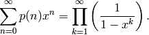
A generating function for p(n) is given by the reciprocal of Euler’s function:

$\sum_{n=0}^\infty p(n)x^n = \prod_{k=1}^\infty \left(\frac {1}{1-x^k} \right).$

We use Sage to verify that the first several coefficients do instead agree:

sage: q = PowerSeriesRing(QQ, 'q', default_prec=9).gen()
sage: prod([(1-q^k)^(-1) for k in range(1,9)])  ## partial product of 
1 + q + 2*q^2 + 3*q^3 + 5*q^4 + 7*q^5 + 11*q^6 + 15*q^7 + 22*q^8 + O(q^9)
sage: [Partitions(k) .cardinality()for k in range(2,10)]
[2, 3, 5, 7, 11, 15, 22, 30]

REFERENCES:

http://en.wikipedia.org/wiki/Partition_(number_theory)

first()¶

Returns the lexicographically first partition of a positive integer n. This is the partition [n].

EXAMPLES:

sage: Partitions(4).first()
[4]

last()¶

Returns the lexicographically last partition of the positive integer n. This is the all-ones partition.

EXAMPLES:

sage: Partitions(4).last()
[1, 1, 1, 1]

random_element(measure='uniform')¶

Returns a random partitions of $n$ for the specified measure.

INPUT:

measure -

uniform - (default) pick a element for the uniform mesure.

see random_element_uniform()

Plancherel - use plancherel measure.

see random_element_plancherel()

EXAMPLES:

sage: Partitions(5).random_element() # random
[2, 1, 1, 1]
sage: Partitions(5).random_element(measure='Plancherel') # random
[2, 1, 1, 1]

random_element_plancherel()¶

Returns a random partitions of $n$ .

EXAMPLES:

sage: Partitions(5).random_element_plancherel()   # random
[2, 1, 1, 1]
sage: Partitions(20).random_element_plancherel()  # random
[9, 3, 3, 2, 2, 1]

TESTS:

sage: all(Part.random_element_plancherel() in Part
...       for Part in map(Partitions, range(10)))
True

ALGORITHM:

insert by robinson-schensted a uniform random permutations of n and returns the shape of the resulting tableau. The complexity is $O(n\ln(n))$ which is likely optimal. However, the implementation could be optimized.

AUTHOR:

Florent Hivert (2009-11-23)

random_element_uniform()¶

Returns a random partitions of $n$ with uniform probability.

EXAMPLES:

sage: Partitions(5).random_element_uniform()  # random
[2, 1, 1, 1]
sage: Partitions(20).random_element_uniform() # random
[9, 3, 3, 2, 2, 1]

TESTS:

sage: all(Part.random_element_uniform() in Part
...       for Part in map(Partitions, range(10)))
True

ALGORITHM:

It is a python Implementation of RANDPAR, see [nw] below. The complexity is unkown, there may be better algorithms. TODO: Check in Knuth AOCP4.

There is also certainly a lot of room for optimizations, see comments in the code.

REFERENCES:

[nw] Nijenhuis, Wilf, Combinatorial Algorithms, Academic Press (1978).

AUTHOR:

Florent Hivert (2009-11-23)

class sage.combinat.partition.Partitions_parts_in(n, parts)¶

Bases: sage.combinat.combinat.CombinatorialClass

Element¶: alias of Partition_class

cardinality()¶

Return the number of partitions with parts in $S$ . Wraps GAP’s NrRestrictedPartitions.

EXAMPLES:

sage: Partitions(15, parts_in=[2,3,7]).cardinality()
5

If you can use all parts 1 through $n$ , we’d better get $p(n)$ :

sage: Partitions(20, parts_in=[1..20]).cardinality() == Partitions(20).cardinality()
True

TESTS:

Let’s check the consistency of GAP’s function and our own algorithm that actually generates the partitions.

sage: ps = Partitions(15, parts_in=[1,2,3])
sage: ps.cardinality() == len(ps.list())
True
sage: ps = Partitions(15, parts_in=[])
sage: ps.cardinality() == len(ps.list())
True
sage: ps = Partitions(3000, parts_in=[50,100,500,1000])
sage: ps.cardinality() == len(ps.list())
True
sage: ps = Partitions(10, parts_in=[3,6,9])
sage: ps.cardinality() == len(ps.list())
True
sage: ps = Partitions(0, parts_in=[1,2])
sage: ps.cardinality() == len(ps.list())
True

first()¶

Return the lexicographically first partition of a positive integer $n$ with the specified parts, or None if no such partition exists.

EXAMPLES:

sage: Partitions(9, parts_in=[3,4]).first()
[3, 3, 3]
sage: Partitions(6, parts_in=[1..6]).first()
[6]
sage: Partitions(30, parts_in=[4,7,8,10,11]).first()
[11, 11, 8]

last()¶

Returns the lexicographically last partition of the positive integer $n$ with the specified parts, or None if no such partition exists.

EXAMPLES:

sage: Partitions(15, parts_in=[2,3]).last()
[3, 2, 2, 2, 2, 2, 2]
sage: Partitions(30, parts_in=[4,7,8,10,11]).last() 
[7, 7, 4, 4, 4, 4]
sage: Partitions(10, parts_in=[3,6]).last() is None
True
sage: Partitions(50, parts_in=[11,12,13]).last()
[13, 13, 12, 12]
sage: Partitions(30, parts_in=[4,7,8,10,11]).last() 
[7, 7, 4, 4, 4, 4]

TESTS:

sage: Partitions(6, parts_in=[1..6]).last()
[1, 1, 1, 1, 1, 1]
sage: Partitions(0, parts_in=[]).last()
[]
sage: Partitions(50, parts_in=[11,12]).last() is None
True

class sage.combinat.partition.Partitions_starting(n, starting_partition)¶

Bases: sage.combinat.combinat.CombinatorialClass

first()¶

EXAMPLES:

sage: Partitions(3, starting=[2,1]).first()
[2, 1]

next(part)¶

EXAMPLES:

sage: Partitions(3, starting=[2,1]).next(Partition([2,1]))
[1, 1, 1]

sage.combinat.partition.RestrictedPartitions(n, S, k=None)¶

This function has been deprecated and will be removed in a future version of Sage; use Partitions() with the parts_in keyword.

Original docstring follows.

A restricted partition is, like an ordinary partition, an unordered sum $n = p_1+p_2+\ldots+p_k$ of positive integers and is represented by the list $p = [p_1,p_2,\ldots,p_k]$ , in nonincreasing order. The difference is that here the $p_i$ must be elements from the set $S$ , while for ordinary partitions they may be elements from $[1..n]$ .

Returns the list of all restricted partitions of the positive integer n into sums with k summands with the summands of the partition coming from the set S. If k is not given all restricted partitions for all k are returned.

Wraps GAP’s RestrictedPartitions.

EXAMPLES:

sage: RestrictedPartitions(5,[3,2,1])
doctest:...: DeprecationWarning: RestrictedPartitions is deprecated; use Partitions with the parts_in keyword instead.
doctest:...: DeprecationWarning: RestrictedPartitions_nsk is deprecated; use Partitions with the parts_in keyword instead.
Partitions of 5 restricted to the values [1, 2, 3] 
sage: RestrictedPartitions(5,[3,2,1]).list()
[[3, 2], [3, 1, 1], [2, 2, 1], [2, 1, 1, 1], [1, 1, 1, 1, 1]]
sage: RestrictedPartitions(5,[3,2,1],4)
Partitions of 5 restricted to the values [1, 2, 3] of length 4
sage: RestrictedPartitions(5,[3,2,1],4).list()
[[2, 1, 1, 1]]

class sage.combinat.partition.RestrictedPartitions_nsk(n, S, k=None)¶

Bases: sage.combinat.combinat.CombinatorialClass

We are deprecating RestrictedPartitions, so this class should be deprecated too.

Element¶: alias of Partition_class

cardinality()¶

Returns the size of RestrictedPartitions(n,S,k). Wraps GAP’s NrRestrictedPartitions.

EXAMPLES:

sage: RestrictedPartitions(8,[1,3,5,7]).cardinality()
doctest:...: DeprecationWarning: RestrictedPartitions is deprecated; use Partitions with the parts_in keyword instead.
6
sage: RestrictedPartitions(8,[1,3,5,7],2).cardinality()
2

list()¶

Returns the list of all restricted partitions of the positive integer n into sums with k summands with the summands of the partition coming from the set $S$ . If k is not given all restricted partitions for all k are returned.

Wraps GAP’s RestrictedPartitions.

EXAMPLES:

sage: RestrictedPartitions(8,[1,3,5,7]).list()
doctest:...: DeprecationWarning: RestrictedPartitions is deprecated; use Partitions with the parts_in keyword instead.
[[7, 1], [5, 3], [5, 1, 1, 1], [3, 3, 1, 1], [3, 1, 1, 1, 1, 1], [1, 1, 1, 1, 1, 1, 1, 1]]
sage: RestrictedPartitions(8,[1,3,5,7],2).list()
[[7, 1], [5, 3]]

sage.combinat.partition.cyclic_permutations_of_partition(partition)¶

Returns all combinations of cyclic permutations of each cell of the partition.

AUTHORS:

Robert L. Miller

EXAMPLES:

sage: from sage.combinat.partition import cyclic_permutations_of_partition         
sage: cyclic_permutations_of_partition([[1,2,3,4],[5,6,7]])
[[[1, 2, 3, 4], [5, 6, 7]],
 [[1, 2, 4, 3], [5, 6, 7]],
 [[1, 3, 2, 4], [5, 6, 7]],
 [[1, 3, 4, 2], [5, 6, 7]],
 [[1, 4, 2, 3], [5, 6, 7]],
 [[1, 4, 3, 2], [5, 6, 7]],
 [[1, 2, 3, 4], [5, 7, 6]],
 [[1, 2, 4, 3], [5, 7, 6]],
 [[1, 3, 2, 4], [5, 7, 6]],
 [[1, 3, 4, 2], [5, 7, 6]],
 [[1, 4, 2, 3], [5, 7, 6]],
 [[1, 4, 3, 2], [5, 7, 6]]]

Note that repeated elements are not considered equal:

sage: cyclic_permutations_of_partition([[1,2,3],[4,4,4]])
[[[1, 2, 3], [4, 4, 4]],
 [[1, 3, 2], [4, 4, 4]],
 [[1, 2, 3], [4, 4, 4]],
 [[1, 3, 2], [4, 4, 4]]]

sage.combinat.partition.cyclic_permutations_of_partition_iterator(partition)¶

Iterates over all combinations of cyclic permutations of each cell of the partition.

AUTHORS:

Robert L. Miller

EXAMPLES:

sage: from sage.combinat.partition import cyclic_permutations_of_partition         
sage: list(cyclic_permutations_of_partition_iterator([[1,2,3,4],[5,6,7]]))
[[[1, 2, 3, 4], [5, 6, 7]],
 [[1, 2, 4, 3], [5, 6, 7]],
 [[1, 3, 2, 4], [5, 6, 7]],
 [[1, 3, 4, 2], [5, 6, 7]],
 [[1, 4, 2, 3], [5, 6, 7]],
 [[1, 4, 3, 2], [5, 6, 7]],
 [[1, 2, 3, 4], [5, 7, 6]],
 [[1, 2, 4, 3], [5, 7, 6]],
 [[1, 3, 2, 4], [5, 7, 6]],
 [[1, 3, 4, 2], [5, 7, 6]],
 [[1, 4, 2, 3], [5, 7, 6]],
 [[1, 4, 3, 2], [5, 7, 6]]]

Note that repeated elements are not considered equal:

sage: list(cyclic_permutations_of_partition_iterator([[1,2,3],[4,4,4]]))
[[[1, 2, 3], [4, 4, 4]],
 [[1, 3, 2], [4, 4, 4]],
 [[1, 2, 3], [4, 4, 4]],
 [[1, 3, 2], [4, 4, 4]]]

sage.combinat.partition.ferrers_diagram(pi)¶

Return the Ferrers diagram of pi.

INPUT:

pi - a partition, given as a list of integers.

EXAMPLES:

sage: print Partition([5,5,2,1]).ferrers_diagram()
*****
*****
**
*        

sage.combinat.partition.from_core_and_quotient(core, quotient)¶

** This function is being deprecated - use Partition(core=*, quotient=*) instead **

Returns a partition from its core and quotient.

Algorithm from mupad-combinat.

Note

This function is for internal use only; use Partition(core=*, quotient=*) instead.

EXAMPLES:

sage: Partition(core=[2,1], quotient=[[2,1],[3],[1,1,1]])
[11, 5, 5, 3, 2, 2, 2]

sage.combinat.partition.from_exp(exp)¶

Returns a partition from its list of multiplicities.

Note

This function is for internal use only; use Partition(exp=*) instead.

EXAMPLES:

sage: Partition(exp=[1,2,1])
[3, 2, 2, 1]

sage.combinat.partition.number_of_ordered_partitions(n, k=None)¶

Returns the size of ordered_partitions(n,k). Wraps GAP’s NrOrderedPartitions.

It is possible to associate with every partition of the integer n a conjugacy class of permutations in the symmetric group on n points and vice versa. Therefore p(n) = NrPartitions(n) is the number of conjugacy classes of the symmetric group on n points.

EXAMPLES:

sage: number_of_ordered_partitions(10,2)
9
sage: number_of_ordered_partitions(15)
16384

sage.combinat.partition.number_of_partitions(n, k=None, algorithm='default')¶

Returns the size of partitions_list(n,k).

INPUT:

n - an integer
k - (default: None); if specified, instead returns the cardinality of the set of all (unordered) partitions of the positive integer n into sums with k summands.
algorithm - (default: ‘default’)
'default' - If k is not None, then use Gap (very slow). If k is None, use Jonathan Bober’s highly optimized implementation (this is the fastest code in the world for this problem).
'bober' - use Jonathan Bober’s implementation
'gap' - use GAP (VERY slow)
'pari' - use PARI. Speed seems the same as GAP until $n$ is in the thousands, in which case PARI is faster. But PARI has a bug, e.g., on 64-bit Linux PARI-2.3.2 outputs numbpart(147007)%1000 as 536 when it should be 533!. So do not use this option.

IMPLEMENTATION: Wraps GAP’s NrPartitions or PARI’s numbpart function.

Use the function partitions(n) to return a generator over all partitions of $n$ .

It is possible to associate with every partition of the integer n a conjugacy class of permutations in the symmetric group on n points and vice versa. Therefore p(n) = NrPartitions(n) is the number of conjugacy classes of the symmetric group on n points.

EXAMPLES:

sage: v = list(partitions(5)); v
[(1, 1, 1, 1, 1), (1, 1, 1, 2), (1, 2, 2), (1, 1, 3), (2, 3), (1, 4), (5,)]
sage: len(v)
7
sage: number_of_partitions(5, algorithm='gap')
7
sage: number_of_partitions(5, algorithm='pari')
7
sage: number_of_partitions(5, algorithm='bober')
7

The input must be a nonnegative integer or a ValueError is raised.

sage: number_of_partitions(-5)
...
ValueError: n (=-5) must be a nonnegative integer

sage: number_of_partitions(10,2)
5
sage: number_of_partitions(10)
42
sage: number_of_partitions(3)
3
sage: number_of_partitions(10)
42
sage: number_of_partitions(3, algorithm='pari')
3
sage: number_of_partitions(10, algorithm='pari')
42
sage: number_of_partitions(40)
37338
sage: number_of_partitions(100)
190569292
sage: number_of_partitions(100000)
27493510569775696512677516320986352688173429315980054758203125984302147328114964173055050741660736621590157844774296248940493063070200461792764493033510116079342457190155718943509725312466108452006369558934464248716828789832182345009262853831404597021307130674510624419227311238999702284408609370935531629697851569569892196108480158600569421098519

A generating function for p(n) is given by the reciprocal of Euler’s function:

$\sum_{n=0}^\infty p(n)x^n = \prod_{k=1}^\infty \left(\frac {1}{1-x^k} \right).$

We use Sage to verify that the first several coefficients do instead agree:

sage: q = PowerSeriesRing(QQ, 'q', default_prec=9).gen()
sage: prod([(1-q^k)^(-1) for k in range(1,9)])  ## partial product of 
1 + q + 2*q^2 + 3*q^3 + 5*q^4 + 7*q^5 + 11*q^6 + 15*q^7 + 22*q^8 + O(q^9)
sage: [number_of_partitions(k) for k in range(2,10)]
[2, 3, 5, 7, 11, 15, 22, 30]

REFERENCES:

http://en.wikipedia.org/wiki/Partition_(number_theory)

TESTS:

sage: n = 500 + randint(0,500)
sage: number_of_partitions( n - (n % 385) + 369) % 385 == 0
True
sage: n = 1500 + randint(0,1500)
sage: number_of_partitions( n - (n % 385) + 369) % 385 == 0
True
sage: n = 1000000 + randint(0,1000000)
sage: number_of_partitions( n - (n % 385) + 369) % 385 == 0
True
sage: n = 1000000 + randint(0,1000000)
sage: number_of_partitions( n - (n % 385) + 369) % 385 == 0
True
sage: n = 1000000 + randint(0,1000000)
sage: number_of_partitions( n - (n % 385) + 369) % 385 == 0
True
sage: n = 1000000 + randint(0,1000000)
sage: number_of_partitions( n - (n % 385) + 369) % 385 == 0
True
sage: n = 1000000 + randint(0,1000000)
sage: number_of_partitions( n - (n % 385) + 369) % 385 == 0
True
sage: n = 1000000 + randint(0,1000000)
sage: number_of_partitions( n - (n % 385) + 369) % 385 == 0
True
sage: n = 100000000 + randint(0,100000000)  
sage: number_of_partitions( n - (n % 385) + 369) % 385 == 0
True
sage: n = 1000000000 + randint(0,1000000000)  
sage: number_of_partitions( n - (n % 385) + 369) % 385 == 0      # takes a long time
True

Another consistency test for n up to 500:

sage: len([n for n in [1..500] if number_of_partitions(n) != number_of_partitions(n,algorithm='pari')])
0

sage.combinat.partition.number_of_partitions_list(n, k=None)¶

This function will be deprecated in a future version of Sage and eventually removed. Use Partitions(n).cardinality() or Partitions(n, length=k).cardinality() instead.

Original docstring follows.

Returns the size of partitions_list(n,k).

Wraps GAP’s NrPartitions.

It is possible to associate with every partition of the integer n a conjugacy class of permutations in the symmetric group on n points and vice versa. Therefore p(n) = NrPartitions(n) is the number of conjugacy classes of the symmetric group on n points.

number_of_partitions(n) is also available in PARI, however the speed seems the same until $n$ is in the thousands (in which case PARI is faster).

EXAMPLES:

sage: partition.number_of_partitions_list(10,2)
5
sage: partition.number_of_partitions_list(10)
42

A generating function for p(n) is given by the reciprocal of Euler’s function:

$\sum_{n=0}^\infty p(n)x^n = \prod_{k=1}^\infty \left(\frac {1}{1-x^k} \right).$

Sage verifies that the first several coefficients do instead agree:

sage: q = PowerSeriesRing(QQ, 'q', default_prec=9).gen()
sage: prod([(1-q^k)^(-1) for k in range(1,9)])  ## partial product of 
1 + q + 2*q^2 + 3*q^3 + 5*q^4 + 7*q^5 + 11*q^6 + 15*q^7 + 22*q^8 + O(q^9)
sage: [partition.number_of_partitions_list(k) for k in range(2,10)]
[2, 3, 5, 7, 11, 15, 22, 30]

REFERENCES:

http://en.wikipedia.org/wiki/Partition_(number_theory)

sage.combinat.partition.number_of_partitions_restricted(n, S, k=None)¶

This function will be deprecated in a future version of Sage and eventually removed. Use RestrictedPartitions(n, S, k).cardinality() instead.

Original docstring follows.

Returns the size of partitions_restricted(n,S,k). Wraps GAP’s NrRestrictedPartitions.

EXAMPLES:

sage: number_of_partitions_restricted(8,[1,3,5,7])
6
sage: number_of_partitions_restricted(8,[1,3,5,7],2)
2

sage.combinat.partition.number_of_partitions_set(S, k)¶

Returns the size of partitions_set(S,k). Wraps GAP’s NrPartitionsSet.

The Stirling number of the second kind is the number of partitions of a set of size n into k blocks.

EXAMPLES:

sage: mset = [1,2,3,4]
sage: number_of_partitions_set(mset,2)
7
sage: stirling_number2(4,2)
7

REFERENCES

http://en.wikipedia.org/wiki/Partition_of_a_set

sage.combinat.partition.number_of_partitions_tuples(n, k)¶

number_of_partition_tuples( n, k ) returns the number of partition_tuples(n,k).

Wraps GAP’s NrPartitionTuples.

EXAMPLES:

sage: number_of_partitions_tuples(3,2)
10
sage: number_of_partitions_tuples(8,2)
185

Now we compare that with the result of the following GAP computation:

gap> S8:=Group((1,2,3,4,5,6,7,8),(1,2));
Group([ (1,2,3,4,5,6,7,8), (1,2) ])
gap> C2:=Group((1,2));
Group([ (1,2) ])
gap> W:=WreathProduct(C2,S8);
<permutation group of size 10321920 with 10 generators>
gap> Size(W);
10321920     ## = 2^8*Factorial(8), which is good:-)
gap> Size(ConjugacyClasses(W));
185

sage.combinat.partition.ordered_partitions(n, k=None)¶

An ordered partition of $n$ is an ordered sum

$n = p_1+p_2 + \cdots + p_k$

of positive integers and is represented by the list $p = [p_1,p_2,\cdots ,p_k]$ . If $k$ is omitted then all ordered partitions are returned.

ordered_partitions(n,k) returns the list of all (ordered) partitions of the positive integer n into sums with k summands.

Do not call ordered_partitions with an n much larger than 15, since the list will simply become too large.

Wraps GAP’s OrderedPartitions.

The number of ordered partitions $T_n$ of $\{ 1, 2, ..., n \}$ has the generating function is

$\sum_n {T_n \over n!} x^n = {1 \over 2-e^x}.$

EXAMPLES:

sage: ordered_partitions(10,2)
[[1, 9], [2, 8], [3, 7], [4, 6], [5, 5], [6, 4], [7, 3], [8, 2], [9, 1]]

sage: ordered_partitions(4)
[[1, 1, 1, 1], [1, 1, 2], [1, 2, 1], [1, 3], [2, 1, 1], [2, 2], [3, 1], [4]]

REFERENCES:

http://en.wikipedia.org/wiki/Ordered_partition_of_a_set

sage.combinat.partition.partition_associated(pi)¶

** This function is being deprecated – use Partition(*).conjugate() instead. **

partition_associated( pi ) returns the “associated” (also called “conjugate” in the literature) partition of the partition pi which is obtained by transposing the corresponding Ferrers diagram.

EXAMPLES:

sage: Partition([2,2]).conjugate()
[2, 2]
sage: Partition([6,3,1]).conjugate()
[3, 2, 2, 1, 1, 1]
sage: print Partition([6,3,1]).ferrers_diagram()
******
***
*
sage: print Partition([6,3,1]).conjugate().ferrers_diagram()
***
**
**
*
*
*

sage.combinat.partition.partition_power(pi, k)¶

partition_power( pi, k ) returns the partition corresponding to the $k$ -th power of a permutation with cycle structure pi (thus describes the powermap of symmetric groups).

Wraps GAP’s PowerPartition.

EXAMPLES:

sage: partition_power([5,3],1)
[5, 3]
sage: partition_power([5,3],2)
[5, 3]
sage: partition_power([5,3],3)
[5, 1, 1, 1]
sage: partition_power([5,3],4)
[5, 3]

Now let us compare this to the power map on $S_8$ :

sage: G = SymmetricGroup(8)
sage: g = G([(1,2,3,4,5),(6,7,8)])
sage: g
(1,2,3,4,5)(6,7,8)
sage: g^2
(1,3,5,2,4)(6,8,7)
sage: g^3
(1,4,2,5,3)
sage: g^4
(1,5,4,3,2)(6,7,8)

sage.combinat.partition.partition_sign(pi)¶

** This function is being deprecated – use Partition(*).sign() instead. **

Partition( pi ).sign() returns the sign of a permutation with cycle structure given by the partition pi.

This function corresponds to a homomorphism from the symmetric group $S_n$ into the cyclic group of order 2, whose kernel is exactly the alternating group $A_n$ . Partitions of sign $1$ are called even partitions while partitions of sign $-1$ are called odd.

This function is deprecated: use Partition( pi ).sign() instead.

EXAMPLES:

sage: Partition([5,3]).sign()
1
sage: Partition([5,2]).sign()
-1

Zolotarev’s lemma states that the Legendre symbol $\left(\frac{a}{p}\right)$ for an integer $a \pmod p$ ( $p$ a prime number), can be computed as sign(p_a), where sign denotes the sign of a permutation and p_a the permutation of the residue classes $\pmod p$ induced by modular multiplication by $a$ , provided $p$ does not divide $a$ .

We verify this in some examples.

sage: F = GF(11)
sage: a = F.multiplicative_generator();a
2
sage: plist = [int(a*F(x)) for x in range(1,11)]; plist
[2, 4, 6, 8, 10, 1, 3, 5, 7, 9]

This corresponds to the permutation (1, 2, 4, 8, 5, 10, 9, 7, 3, 6) (acting the set $\{1,2,...,10\}$ ) and to the partition [10].

sage: p = PermutationGroupElement('(1, 2, 4, 8, 5, 10, 9, 7, 3, 6)')
sage: p.sign()
-1
sage: Partition([10]).sign()
-1
sage: kronecker_symbol(11,2)
-1

Now replace $2$ by $3$ :

sage: plist = [int(F(3*x)) for x in range(1,11)]; plist
[3, 6, 9, 1, 4, 7, 10, 2, 5, 8]
sage: range(1,11)
[1, 2, 3, 4, 5, 6, 7, 8, 9, 10]
sage: p = PermutationGroupElement('(3,4,8,7,9)')
sage: p.sign()
1
sage: kronecker_symbol(3,11)
1
sage: Partition([5,1,1,1,1,1]).sign()
1

In both cases, Zolotarev holds.

REFERENCES:

http://en.wikipedia.org/wiki/Zolotarev’s_lemma

sage.combinat.partition.partitions(n)¶

Generator of all the partitions of the integer $n$ .

INPUT:

n - int

To compute the number of partitions of $n$ use number_of_partitions(n).

EXAMPLES:

sage: partitions(3)
<generator object partitions at 0x...>
sage: list(partitions(3))
[(1, 1, 1), (1, 2), (3,)]

AUTHORS:

Adapted from David Eppstein, Jan Van lent, George Yoshida; Python Cookbook 2, Recipe 19.16.

sage.combinat.partition.partitions_greatest(n, k)¶

Returns the list of all (unordered) “restricted” partitions of the integer n having parts less than or equal to the integer k.

Wraps GAP’s PartitionsGreatestLE.

EXAMPLES:

sage: partitions_greatest(10,2)
[[1, 1, 1, 1, 1, 1, 1, 1, 1, 1],
 [2, 1, 1, 1, 1, 1, 1, 1, 1],
 [2, 2, 1, 1, 1, 1, 1, 1],
 [2, 2, 2, 1, 1, 1, 1],
 [2, 2, 2, 2, 1, 1],
 [2, 2, 2, 2, 2]]

sage.combinat.partition.partitions_greatest_eq(n, k)¶

Returns the list of all (unordered) “restricted” partitions of the integer n having at least one part equal to the integer k.

Wraps GAP’s PartitionsGreatestEQ.

EXAMPLES:

sage: partitions_greatest_eq(10,2)
[[2, 1, 1, 1, 1, 1, 1, 1, 1],
 [2, 2, 1, 1, 1, 1, 1, 1],
 [2, 2, 2, 1, 1, 1, 1],
 [2, 2, 2, 2, 1, 1],
 [2, 2, 2, 2, 2]]

sage.combinat.partition.partitions_list(n, k=None)¶

This function will be deprecated in a future version of Sage and eventually removed. Use Partitions(n).list() or Partitions(n, length=k).list() instead.

Original docstring follows.

An unordered partition of $n$ is an unordered sum $n = p_1+p_2 +\ldots+ p_k$ of positive integers and is represented by the list $p = [p_1,p_2,\ldots,p_k]$ , in nonincreasing order, i.e., $p1\geq p_2 ...\geq p_k$ .

INPUT:

n, k - positive integer

partitions_list(n,k) returns the list of all (unordered) partitions of the positive integer n into sums with k summands. If k is omitted then all partitions are returned.

Do not call partitions_list with an n much larger than 40, in which case there are 37338 partitions, since the list will simply become too large.

Wraps GAP’s Partitions.

EXAMPLES:

sage: partitions_list(10,2)
[[5, 5], [6, 4], [7, 3], [8, 2], [9, 1]]
sage: partitions_list(5)
[[1, 1, 1, 1, 1], [2, 1, 1, 1], [2, 2, 1], [3, 1, 1], [3, 2], [4, 1], [5]]

sage.combinat.partition.partitions_restricted(n, S, k=None)¶

This function will be deprecated in a future version of Sage and eventually removed. Use RestrictedPartitions(n, S, k).list() instead.

Original docstring follows.

A restricted partition is, like an ordinary partition, an unordered sum $n = p_1+p_2+\ldots+p_k$ of positive integers and is represented by the list $p = [p_1,p_2,\ldots,p_k]$ , in nonincreasing order. The difference is that here the $p_i$ must be elements from the set $S$ , while for ordinary partitions they may be elements from $[1..n]$ .

Returns the list of all restricted partitions of the positive integer n into sums with k summands with the summands of the partition coming from the set $S$ . If k is not given all restricted partitions for all k are returned.

Wraps GAP’s RestrictedPartitions.

EXAMPLES:

sage: partitions_restricted(8,[1,3,5,7])
[[1, 1, 1, 1, 1, 1, 1, 1],
 [3, 1, 1, 1, 1, 1],
 [3, 3, 1, 1],
 [5, 1, 1, 1],
 [5, 3],
 [7, 1]]
sage: partitions_restricted(8,[1,3,5,7],2)
[[5, 3], [7, 1]]

sage.combinat.partition.partitions_set(S, k=None, use_file=True)¶

An unordered partition of a set $S$ is a set of pairwise disjoint nonempty subsets with union $S$ and is represented by a sorted list of such subsets.

partitions_set returns the list of all unordered partitions of the list $S$ of increasing positive integers into k pairwise disjoint nonempty sets. If k is omitted then all partitions are returned.

The Bell number $B_n$ , named in honor of Eric Temple Bell, is the number of different partitions of a set with n elements.

Warning

Wraps GAP - hence S must be a list of objects that have string representations that can be interpreted by the GAP interpreter. If mset consists of at all complicated Sage objects, this function does not do what you expect. See SetPartitions in combinat/set_partition.

Warning

This function is inefficient. The runtime is dominated by parsing the output from GAP.

Wraps GAP’s PartitionsSet.

EXAMPLES:

sage: S = [1,2,3,4]
sage: partitions_set(S,2)
[[[1], [2, 3, 4]],
 [[1, 2], [3, 4]],
 [[1, 2, 3], [4]],
 [[1, 2, 4], [3]],
 [[1, 3], [2, 4]],
 [[1, 3, 4], [2]],
 [[1, 4], [2, 3]]]

REFERENCES:

http://en.wikipedia.org/wiki/Partition_of_a_set

sage.combinat.partition.partitions_tuples(n, k)¶

partition_tuples( n, k ) returns the list of all k-tuples of partitions which together form a partition of n.

k-tuples of partitions describe the classes and the characters of wreath products of groups with k conjugacy classes with the symmetric group $S_n$ .

Wraps GAP’s PartitionTuples.

EXAMPLES:

sage: partitions_tuples(3,2)
[[[1, 1, 1], []],
 [[1, 1], [1]],
 [[1], [1, 1]],
 [[], [1, 1, 1]],
 [[2, 1], []],
 [[1], [2]],
 [[2], [1]],
 [[], [2, 1]],
 [[3], []],
 [[], [3]]]

Partitions¶

Previous topic

Next topic

This Page

Navigation

Partitions¶

Previous topic

Next topic

This Page

Quick search

Navigation