Symbolic Expressions¶

RELATIONAL EXPRESSIONS:

We create a relational expression:

sage: x = var('x')
sage: eqn = (x-1)^2 <= x^2 - 2*x + 3
sage: eqn.subs(x == 5)
16 <= 18

Notice that squaring the relation squares both sides.

sage: eqn^2
(x - 1)^4 <= (x^2 - 2*x + 3)^2
sage: eqn.expand()
x^2 - 2*x + 1 <= x^2 - 2*x + 3

The can transform a true relational into a false one:

sage: eqn = SR(-5) < SR(-3); eqn
-5 < -3
sage: bool(eqn)
True
sage: eqn^2
25 < 9
sage: bool(eqn^2)
False

We can do arithmetic with relationals:

sage: e = x+1 <= x-2
sage: e + 2
x + 3 <= x
sage: e - 1
x <= x - 3
sage: e*(-1)
-x - 1 <= -x + 2
sage: (-2)*e
-2*x - 2 <= -2*x + 4
sage: e*5
5*x + 5 <= 5*x - 10
sage: e/5
1/5*x + 1/5 <= 1/5*x - 2/5
sage: 5/e
5/(x + 1) <= 5/(x - 2)
sage: e/(-2)
-1/2*x - 1/2 <= -1/2*x + 1
sage: -2/e
-2/(x + 1) <= -2/(x - 2)

We can even add together two relations, so long as the operators are the same:

sage: (x^3 + x <= x - 17)  + (-x <= x - 10)
x^3 <= 2*x - 27

Here they aren’t:

sage: (x^3 + x <= x - 17)  + (-x >= x - 10)
...
TypeError: incompatible relations

ARBITRARY SAGE ELEMENTS:

You can work symbolically with any Sage data type. This can lead to nonsense if the data type is strange, e.g., an element of a finite field (at present).

We mix Singular variables with symbolic variables:

sage: R.<u,v> = QQ[]
sage: var('a,b,c')
(a, b, c)
sage: expand((u + v + a + b + c)^2)
a^2 + 2*a*b + 2*a*c + 2*a*u + 2*a*v + b^2 + 2*b*c + 2*b*u + 2*b*v + c^2 + 2*c*u + 2*c*v + u^2 + 2*u*v + v^2

TESTS:

Test Jacobian on Pynac expressions. #5546

sage: var('x,y')
(x, y)
sage: f = x + y
sage: jacobian(f, [x,y])
[1 1]

Test if matrices work #5546

sage: var('x,y,z')
(x, y, z)
sage: M = matrix(2,2,[x,y,z,x])
sage: v = vector([x,y])
sage: M * v
(x^2 + y^2, x*y + x*z)
sage: v*M
(x^2 + y*z, 2*x*y)

Test if comparison bugs from #6256 are fixed:

sage: t = exp(sqrt(x)); u = 1/t
sage: t*u
1
sage: t + u
e^sqrt(x) + e^(-sqrt(x))
sage: t
e^sqrt(x)

class sage.symbolic.expression.Expression¶

Bases: sage.structure.element.CommutativeRingElement

Order()¶

Order, as in big oh notation.

OUTPUT:: symbolic expression
EXAMPLES:: sage: n = var(‘n’) sage: t = (17*n^3).Order(); t Order(n^3) sage: t.derivative(n) Order(n^2)

add_to_both_sides(x)¶

Returns a relation obtained by adding x to both sides of this relation.

EXAMPLES:

sage: var('x y z')
(x, y, z)
sage: eqn = x^2 + y^2 + z^2 <= 1
sage: eqn.add_to_both_sides(-z^2)
x^2 + y^2 <= -z^2 + 1
sage: eqn.add_to_both_sides(I)
x^2 + y^2 + z^2 + I <= (I + 1)

arccos()¶

Return the arc cosine of self.

EXAMPLES:

sage: x.arccos()
arccos(x)
sage: SR(1).arccos()
0
sage: SR(1/2).arccos()
1/3*pi
sage: SR(0.4).arccos()
1.15927948072741
sage: plot(lambda x: SR(x).arccos(), -1,1)

TESTS:

sage: SR(oo).arccos()
...
RuntimeError: arccos_eval(): arccos(infinity) encountered
sage: SR(-oo).arccos()
...
RuntimeError: arccos_eval(): arccos(infinity) encountered
sage: SR(unsigned_infinity).arccos()
Infinity

arccosh()¶

Return the inverse hyperbolic cosine of self.

EXAMPLES:

sage: x.arccosh()
arccosh(x)
sage: SR(0).arccosh()
1/2*I*pi
sage: SR(1/2).arccosh()
arccosh(1/2)
sage: SR(CDF(1/2)).arccosh()
1.0471975512*I
sage: maxima('acosh(0.5)')
1.047197551196598*%i

TESTS:

sage: SR(oo).arccosh()
+Infinity
sage: SR(-oo).arccosh()
+Infinity
sage: SR(unsigned_infinity).arccosh()
+Infinity

arcsin()¶

Return the arcsin of x, i.e., the number y between -pi and pi such that sin(y) == x.

EXAMPLES:

sage: x.arcsin()
arcsin(x)
sage: SR(0.5).arcsin()
0.523598775598299
sage: SR(0.999).arcsin()
1.52607123962616
sage: SR(1/3).arcsin()
arcsin(1/3)
sage: SR(-1/3).arcsin()
-arcsin(1/3)

TESTS:

sage: SR(oo).arcsin()
...
RuntimeError: arcsin_eval(): arcsin(infinity) encountered
sage: SR(-oo).arcsin()
...
RuntimeError: arcsin_eval(): arcsin(infinity) encountered
sage: SR(unsigned_infinity).arcsin()
Infinity

arcsinh()¶

Return the inverse hyperbolic sine of self.

EXAMPLES:

sage: x.arcsinh()
arcsinh(x)
sage: SR(0).arcsinh()
0
sage: SR(1).arcsinh()
arcsinh(1)
sage: SR(1.0).arcsinh()
0.881373587019543
sage: maxima('asinh(1.0)')
0.881373587019543

Sage automatically applies certain identities::: sage: SR(3/2).arcsinh().cosh() 1/2*sqrt(13)

TESTS:

sage: SR(oo).arcsinh()
+Infinity
sage: SR(-oo).arcsinh()
-Infinity
sage: SR(unsigned_infinity).arcsinh()
Infinity

arctan()¶

Return the arc tangent of self.

EXAMPLES:

sage: x = var('x')
sage: x.arctan()
arctan(x)
sage: SR(1).arctan()
1/4*pi
sage: SR(1/2).arctan()
arctan(1/2)
sage: SR(0.5).arctan()
0.463647609000806
sage: plot(lambda x: SR(x).arctan(), -20,20)

TESTS:

sage: SR(oo).arctan()
1/2*pi
sage: SR(-oo).arctan()
-1/2*pi
sage: SR(unsigned_infinity).arctan()
...
RuntimeError: arctan_eval(): arctan(unsigned_infinity) encountered

arctan2(x)¶

Return the inverse of the 2-variable tan function on self and x.

EXAMPLES:

sage: var('x,y')
(x, y)
sage: x.arctan2(y)
arctan2(x, y)
sage: SR(1/2).arctan2(1/2)
1/4*pi
sage: maxima.eval('atan2(1/2,1/2)')
'%pi/4'

sage: SR(-0.7).arctan2(SR(-0.6))
-pi + 0.862170054667226

TESTS:

We compare a bunch of different evaluation points between Sage and Maxima:

sage: float(SR(0.7).arctan2(0.6))
0.8621700546672264
sage: maxima('atan2(0.7,0.6)')
.862170054667226...
sage: float(SR(0.7).arctan2(-0.6))
2.2794225989225669
sage: maxima('atan2(0.7,-0.6)')
2.279422598922567
sage: float(SR(-0.7).arctan2(0.6))
-0.8621700546672264
sage: maxima('atan2(-0.7,0.6)')
-.862170054667226...
sage: float(SR(-0.7).arctan2(-0.6))
-2.2794225989225669
sage: maxima('atan2(-0.7,-0.6)')
-2.279422598922567
sage: float(SR(0).arctan2(-0.6))
3.1415926535897931
sage: maxima('atan2(0,-0.6)')
3.141592653589793
sage: float(SR(0).arctan2(0.6))
0.0
sage: maxima('atan2(0,0.6)')
0.0
sage: SR(0).arctan2(0)
0

sage: SR(I).arctan2(1)
arctan2(I, 1)
sage: SR(CDF(0,1)).arctan2(1)
arctan2(1.0*I, 1)
sage: SR(1).arctan2(CDF(0,1))
arctan2(1, 1.0*I)

sage: SR(oo).arctan2(oo)
...
RuntimeError: arctan2_eval(): arctan2(infinity, infinity) encountered
sage: SR(oo).arctan2(0)
0
sage: SR(-oo).arctan2(0)
pi
sage: SR(-oo).arctan2(-2)
-pi
sage: SR(unsigned_infinity).arctan2(2)
...
RuntimeError: arctan2_eval(): arctan2(unsigned_infinity, x) encountered
sage: SR(2).arctan2(oo)
1/2*pi
sage: SR(2).arctan2(-oo)
-1/2*pi
sage: SR(2).arctan2(SR(unsigned_infinity))
...
RuntimeError: arctan2_eval(): arctan2(x, unsigned_infinity) encountered

arctanh()¶

Return the inverse hyperbolic tangent of self.

EXAMPLES:

sage: x.arctanh()
arctanh(x)
sage: SR(0).arctanh()
0
sage: SR(1/2).arctanh()
arctanh(1/2)
sage: SR(0.5).arctanh()
0.549306144334055
sage: SR(0.5).arctanh().tanh()
0.500000000000000
sage: maxima('atanh(0.5)')
.5493061443340...

TESTS:

sage: SR(1).arctanh()
+Infinity
sage: SR(-1).arctanh()
-Infinity

sage: SR(oo).arctanh()
-1/2*I*pi
sage: SR(-oo).arctanh()
1/2*I*pi
sage: SR(unsigned_infinity).arctanh()
...
RuntimeError: arctanh_eval(): arctanh(unsigned_infinity) encountered

args()¶

EXAMPLES:

sage: x,y = var('x,y')
sage: f = x + y
sage: f.arguments()
(x, y)

sage: g = f.function(x)
sage: g.arguments()
(x,)

arguments()¶

EXAMPLES:

sage: x,y = var('x,y')
sage: f = x + y
sage: f.arguments()
(x, y)

sage: g = f.function(x)
sage: g.arguments()
(x,)

assume()¶

Assume that this equation holds. This is relevant for symbolic integration, among other things.

EXAMPLES: We call the assume method to assume that $x>2$ :

sage: (x > 2).assume()

Bool returns True below if the inequality is definitely known to be True.

sage: bool(x > 0)
True
sage: bool(x < 0)
False

This may or may not be True, so bool returns False:

sage: bool(x > 3)
False

If you make inconsistent or meaningless assumptions, Sage will let you know:

sage: forget()
sage: assume(x<0)
sage: assume(x>0)
...
ValueError: Assumption is inconsistent
sage: assumptions()
[x < 0]
sage: forget()

TESTS:

sage: v,c = var('v,c')
sage: assume(c != 0)
sage: integral((1+v^2/c^2)^3/(1-v^2/c^2)^(3/2),v)
-75/8*sqrt(c^2)*arcsin(sqrt(c^2)*v/c^2) - 17/8*v^3/(sqrt(-v^2/c^2 + 1)*c^2) - 1/4*v^5/(sqrt(-v^2/c^2 + 1)*c^4) + 83/8*v/sqrt(-v^2/c^2 + 1)
sage: forget()

binomial(k)¶

Return binomial coefficient “self choose k”.

OUTPUT:: symbolic expression
EXAMPLES:: sage: var(‘x, y’) (x, y) sage: SR(5).binomial(SR(3)) 10 sage: x.binomial(SR(3)) 1/6*x^3 - 1/2*x^2 + 1/3*x sage: x.binomial(y) binomial(x, y)

TESTS:

Check if we handle zero correctly (#8561)::: sage: x.binomial(0) 1 sage: SR(0).binomial(0) 1

coeff(s, n=1)¶

Returns the coefficient of $s^n$ in this symbolic expression.

INPUT:

s - expression
n - integer, default 1

OUTPUT:

coefficient of s^n

Sometimes it may be necessary to expand or factor first, since this is not done automatically.

EXAMPLES:

sage: var('x,y,a')
(x, y, a)
sage: f = 100 + a*x + x^3*sin(x*y) + x*y + x/y + 2*sin(x*y)/x; f
x^3*sin(x*y) + a*x + x*y + x/y + 2*sin(x*y)/x + 100
sage: f.collect(x)
x^3*sin(x*y) + (a + y + 1/y)*x + 2*sin(x*y)/x + 100
sage: f.coefficient(x,0)
100
sage: f.coefficient(x,-1)
2*sin(x*y)
sage: f.coefficient(x,1)
a + y + 1/y
sage: f.coefficient(x,2)
0
sage: f.coefficient(x,3)
sin(x*y)
sage: f.coefficient(x^3)
sin(x*y)
sage: f.coefficient(sin(x*y))
x^3 + 2/x
sage: f.collect(sin(x*y))
(x^3 + 2/x)*sin(x*y) + a*x + x*y + x/y + 100

sage: var('a, x, y, z')
(a, x, y, z)
sage: f = (a*sqrt(2))*x^2 + sin(y)*x^(1/2) + z^z   
sage: f.coefficient(sin(y))
sqrt(x)        
sage: f.coefficient(x^2)
sqrt(2)*a
sage: f.coefficient(x^(1/2))
sin(y)
sage: f.coefficient(1)
0
sage: f.coefficient(x, 0)
sqrt(x)*sin(y) + z^z

coefficient(s, n=1)¶

Returns the coefficient of $s^n$ in this symbolic expression.

INPUT:

s - expression
n - integer, default 1

OUTPUT:

coefficient of s^n

Sometimes it may be necessary to expand or factor first, since this is not done automatically.

EXAMPLES:

sage: var('x,y,a')
(x, y, a)
sage: f = 100 + a*x + x^3*sin(x*y) + x*y + x/y + 2*sin(x*y)/x; f
x^3*sin(x*y) + a*x + x*y + x/y + 2*sin(x*y)/x + 100
sage: f.collect(x)
x^3*sin(x*y) + (a + y + 1/y)*x + 2*sin(x*y)/x + 100
sage: f.coefficient(x,0)
100
sage: f.coefficient(x,-1)
2*sin(x*y)
sage: f.coefficient(x,1)
a + y + 1/y
sage: f.coefficient(x,2)
0
sage: f.coefficient(x,3)
sin(x*y)
sage: f.coefficient(x^3)
sin(x*y)
sage: f.coefficient(sin(x*y))
x^3 + 2/x
sage: f.collect(sin(x*y))
(x^3 + 2/x)*sin(x*y) + a*x + x*y + x/y + 100

sage: var('a, x, y, z')
(a, x, y, z)
sage: f = (a*sqrt(2))*x^2 + sin(y)*x^(1/2) + z^z   
sage: f.coefficient(sin(y))
sqrt(x)        
sage: f.coefficient(x^2)
sqrt(2)*a
sage: f.coefficient(x^(1/2))
sin(y)
sage: f.coefficient(1)
0
sage: f.coefficient(x, 0)
sqrt(x)*sin(y) + z^z

coefficients(x=None)¶

Coefficients of this symbolic expression as a polynomial in x.

INPUT:

x - optional variable

OUTPUT:

A list of pairs (expr, n), where expr is a symbolic expression and n is a power.

EXAMPLES:

sage: var('x, y, a')
(x, y, a)
sage: p = x^3 - (x-3)*(x^2+x) + 1
sage: p.coefficients()
[[1, 0], [3, 1], [2, 2]]
sage: p = expand((x-a*sqrt(2))^2 + x + 1); p
-2*sqrt(2)*a*x + 2*a^2 + x^2 + x + 1
sage: p.coefficients(a)
[[x^2 + x + 1, 0], [-2*sqrt(2)*x, 1], [2, 2]]
sage: p.coefficients(x)
[[2*a^2 + 1, 0], [-2*sqrt(2)*a + 1, 1], [1, 2]]

A polynomial with wacky exponents:

sage: p = (17/3*a)*x^(3/2) + x*y + 1/x + x^x
sage: p.coefficients(x)
[[1, -1], [x^x, 0], [y, 1], [17/3*a, 3/2]]

coeffs(x=None)¶

Coefficients of this symbolic expression as a polynomial in x.

INPUT:

x - optional variable

OUTPUT:

A list of pairs (expr, n), where expr is a symbolic expression and n is a power.

EXAMPLES:

sage: var('x, y, a')
(x, y, a)
sage: p = x^3 - (x-3)*(x^2+x) + 1
sage: p.coefficients()
[[1, 0], [3, 1], [2, 2]]
sage: p = expand((x-a*sqrt(2))^2 + x + 1); p
-2*sqrt(2)*a*x + 2*a^2 + x^2 + x + 1
sage: p.coefficients(a)
[[x^2 + x + 1, 0], [-2*sqrt(2)*x, 1], [2, 2]]
sage: p.coefficients(x)
[[2*a^2 + 1, 0], [-2*sqrt(2)*a + 1, 1], [1, 2]]

A polynomial with wacky exponents:

sage: p = (17/3*a)*x^(3/2) + x*y + 1/x + x^x
sage: p.coefficients(x)
[[1, -1], [x^x, 0], [y, 1], [17/3*a, 3/2]]

collect(s)¶

INPUT:

s - a symbol

OUTPUT:

expression

EXAMPLES:

sage: var('x,y,z')
(x, y, z)
sage: f = 4*x*y + x*z + 20*y^2 + 21*y*z + 4*z^2 + x^2*y^2*z^2
sage: f.collect(x)
x^2*y^2*z^2 + (4*y + z)*x + 20*y^2 + 21*y*z + 4*z^2
sage: f.collect(y)
(x^2*z^2 + 20)*y^2 + (4*x + 21*z)*y + x*z + 4*z^2
sage: f.collect(z)
(x^2*y^2 + 4)*z^2 + (x + 21*y)*z + 4*x*y + 20*y^2

collect_common_factors()¶

EXAMPLES:

sage: var('x')
x
sage: (x/(x^2 + x)).collect_common_factors()
1/(x + 1)

combine()¶

Returns a simplified version of this symbolic expression by combining all terms with the same denominator into a single term.

EXAMPLES:

sage: var('x, y, a, b, c')
(x, y, a, b, c)
sage: f = x*(x-1)/(x^2 - 7) + y^2/(x^2-7) + 1/(x+1) + b/a + c/a; f
(x - 1)*x/(x^2 - 7) + y^2/(x^2 - 7) + b/a + c/a + 1/(x + 1)
sage: f.combine()
((x - 1)*x + y^2)/(x^2 - 7) + (b + c)/a + 1/(x + 1)

conjugate()¶

Return the complex conjugate of this symbolic expression.

EXAMPLES:

sage: a = 1 + 2*I 
sage: a.conjugate()
-2*I + 1
sage: a = sqrt(2) + 3^(1/3)*I; a
sqrt(2) + I*3^(1/3)
sage: a.conjugate()
sqrt(2) - I*3^(1/3)

sage: SR(CDF.0).conjugate()
-1.0*I
sage: x.conjugate()
conjugate(x)
sage: SR(RDF(1.5)).conjugate()
1.5
sage: SR(float(1.5)).conjugate()
1.5
sage: SR(I).conjugate()
-I
sage: ( 1+I  + (2-3*I)*x).conjugate()
(3*I + 2)*conjugate(x) - I + 1

contradicts(soln)¶

Returns True if this relation is violated by the given variable assignment(s).

EXAMPLES:

sage: (x<3).contradicts(x==0)
False
sage: (x<3).contradicts(x==3)
True
sage: (x<=3).contradicts(x==3)
False
sage: y = var('y')
sage: (x<y).contradicts(x==30)
False
sage: (x<y).contradicts({x: 30, y: 20})
True

convert(target=None)¶

Calls the convert function in the units package. For symbolic variables that are not units, this function just returns the variable.

INPUT:

$self$ – the symbolic expression converting from

$target$ – (default None) the symbolic expression converting to

OUTPUT:

$symbolic expression$

EXAMPLES:

sage: units.length.foot.convert()
381/1250*meter
sage: units.mass.kilogram.convert(units.mass.pound)
100000000/45359237*pound

We don’t get anything new by converting an ordinary symbolic variable:

sage: a = var('a')
sage: a - a.convert()
0

Raises ValueError if self and target are not convertible:

sage: units.mass.kilogram.convert(units.length.foot)
...
ValueError: Incompatible units
sage: (units.length.meter^2).convert(units.length.foot)
...
ValueError: Incompatible units

Recognizes derived unit relationships to base units and other derived units:

sage: (units.length.foot/units.time.second^2).convert(units.acceleration.galileo)
762/25*galileo
sage: (units.mass.kilogram*units.length.meter/units.time.second^2).convert(units.force.newton)
newton
sage: (units.length.foot^3).convert(units.area.acre*units.length.inch)
1/3630*acre*inch
sage: (units.charge.coulomb).convert(units.current.ampere*units.time.second)
ampere*second
sage: (units.pressure.pascal*units.si_prefixes.kilo).convert(units.pressure.pounds_per_square_inch)
1290320000000/8896443230521*pounds_per_square_inch

For decimal answers multiply by 1.0:

sage: (units.pressure.pascal*units.si_prefixes.kilo).convert(units.pressure.pounds_per_square_inch)*1.0
0.145037737730209*pounds_per_square_inch

Converting temperatures works as well:

sage: s = 68*units.temperature.fahrenheit
sage: s.convert(units.temperature.celsius)
20*celsius
sage: s.convert()
293.150000000000*kelvin

Trying to multiply temperatures by another unit then converting raises a ValueError:

sage: wrong = 50*units.temperature.celsius*units.length.foot
sage: wrong.convert()
...
ValueError: Cannot convert

cos()¶

Return the cosine of self.

EXAMPLES:

sage: var('x, y')
(x, y)
sage: cos(x^2 + y^2)
cos(x^2 + y^2)
sage: cos(sage.symbolic.constants.pi)
-1
sage: cos(SR(1))
cos(1)
sage: cos(SR(RealField(150)(1)))
0.54030230586813971740093660744297660373231042

In order to get a numeric approximation use .n():

sage: SR(RR(1)).cos().n()
0.540302305868140
sage: SR(float(1)).cos().n()
0.540302305868140            

TESTS:

sage: SR(oo).cos()
...
RuntimeError: cos_eval(): cos(infinity) encountered
sage: SR(-oo).cos()
...
RuntimeError: cos_eval(): cos(infinity) encountered
sage: SR(unsigned_infinity).cos()
...
RuntimeError: cos_eval(): cos(infinity) encountered

cosh()¶

Return cosh of self.

We have 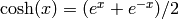$\cosh(x) = (e^{x} + e^{-x})/2$ .

EXAMPLES:

sage: x.cosh()
cosh(x)
sage: SR(1).cosh()
cosh(1)
sage: SR(0).cosh()
1
sage: SR(1.0).cosh()
1.54308063481524
sage: maxima('cosh(1.0)')
1.543080634815244
sage: SR(1.00000000000000000000000000).cosh()
1.5430806348152437784779056
sage: SR(RIF(1)).cosh()
1.543080634815244?

TESTS:

sage: SR(oo).cosh()
+Infinity
sage: SR(-oo).cosh()
+Infinity
sage: SR(unsigned_infinity).cosh()
...
RuntimeError: cosh_eval(): cosh(unsigned_infinity) encountered

csgn()¶

Return the sign of self, which is -1 if self < 0, 0 if self == 0, and 1 if self > 0, or unevaluated when self is a nonconstant symbolic expression.

It can be somewhat arbitrary when self is not real.

EXAMPLES:: sage: x = var(‘x’) sage: SR(-2).csgn() -1 sage: SR(0.0).csgn() 0 sage: SR(10).csgn() 1 sage: x.csgn() csgn(x) sage: SR(CDF.0).csgn() 1 sage: SR(I).csgn() 1

default_variable()¶

Return the default variable, which is by definition the first variable in self, or $x$ is there are no variables in self. The result is cached.

EXAMPLES:

sage: sqrt(2).default_variable()
x        
sage: x, theta, a = var('x, theta, a')
sage: f = x^2 + theta^3 - a^x
sage: f.default_variable()
a

Note that this is the first variable, not the first argument:

sage: f(theta, a, x) = a + theta^3
sage: f.default_variable()
a
sage: f.variables()
(a, theta)
sage: f.arguments()
(theta, a, x)

degree(s)¶

Return the exponent of the highest nonnegative power of s in self.

OUTPUT:

an integer >= 0.

EXAMPLES:

sage: var('x,y,a')
(x, y, a)
sage: f = 100 + a*x + x^3*sin(x*y) + x*y + x/y^10 + 2*sin(x*y)/x; f
x^3*sin(x*y) + a*x + x*y + 2*sin(x*y)/x + x/y^10 + 100
sage: f.degree(x)
3
sage: f.degree(y)
1
sage: f.degree(sin(x*y))
1
sage: (x^-3+y).degree(x)
0

denominator()¶

Returns the denominator of this symbolic expression. If the expression is not a quotient, then this will just return 1.

EXAMPLES:

sage: x, y, z, theta = var('x, y, z, theta')
sage: f = (sqrt(x) + sqrt(y) + sqrt(z))/(x^10 - y^10 - sqrt(theta))
sage: f.denominator()
sqrt(theta) - x^10 + y^10

sage: y = var('y')
sage: g = x + y/(x + 2); g
x + y/(x + 2)
sage: g.numerator()
x + y/(x + 2)
sage: g.denominator()
1

derivative(*args)¶

Returns the derivative of this expressions with respect to the variables supplied in args.

Multiple variables and iteration counts may be supplied; see documentation for the global derivative() function for more details.

See also

_derivative()

EXAMPLES:

sage: var("x y")
(x, y)
sage: t = (x^2+y)^2
sage: t.derivative(x)
4*(x^2 + y)*x
sage: t.derivative(x, 2)
12*x^2 + 4*y
sage: t.derivative(x, 2, y)
4
sage: t.derivative(y)
2*x^2 + 2*y

sage: t = sin(x+y^2)*tan(x*y)
sage: t.derivative(x)
(tan(x*y)^2 + 1)*y*sin(y^2 + x) + cos(y^2 + x)*tan(x*y)
sage: t.derivative(y)
(tan(x*y)^2 + 1)*x*sin(y^2 + x) + 2*y*cos(y^2 + x)*tan(x*y)

sage: h = sin(x)/cos(x)
sage: derivative(h,x,x,x)
6*sin(x)^4/cos(x)^4 + 8*sin(x)^2/cos(x)^2 + 2
sage: derivative(h,x,3)
6*sin(x)^4/cos(x)^4 + 8*sin(x)^2/cos(x)^2 + 2

sage: var('x, y')
(x, y)
sage: u = (sin(x) + cos(y))*(cos(x) - sin(y))
sage: derivative(u,x,y)
sin(x)*sin(y) - cos(x)*cos(y)            
sage: f = ((x^2+1)/(x^2-1))^(1/4)
sage: g = derivative(f, x); g # this is a complex expression
1/2*(x/(x^2 - 1) - (x^2 + 1)*x/(x^2 - 1)^2)/((x^2 + 1)/(x^2 - 1))^(3/4)
sage: g.factor()
-x/((x^2 - 1)^(5/4)*(x^2 + 1)^(3/4))

sage: y = var('y')
sage: f = y^(sin(x))
sage: derivative(f, x)
y^sin(x)*log(y)*cos(x)

sage: g(x) = sqrt(5-2*x)
sage: g_3 = derivative(g, x, 3); g_3(2)
-3

sage: f = x*e^(-x)
sage: derivative(f, 100)
x*e^(-x) - 100*e^(-x)

sage: g = 1/(sqrt((x^2-1)*(x+5)^6))
sage: derivative(g, x)
-((x + 5)^6*x + 3*(x + 5)^5*(x^2 - 1))/((x + 5)^6*(x^2 - 1))^(3/2)

TESTS:

sage: t.derivative()
...
ValueError: No differentiation variable specified.

diff(*args)¶

Returns the derivative of this expressions with respect to the variables supplied in args.

Multiple variables and iteration counts may be supplied; see documentation for the global derivative() function for more details.

See also

_derivative()

EXAMPLES:

sage: var("x y")
(x, y)
sage: t = (x^2+y)^2
sage: t.derivative(x)
4*(x^2 + y)*x
sage: t.derivative(x, 2)
12*x^2 + 4*y
sage: t.derivative(x, 2, y)
4
sage: t.derivative(y)
2*x^2 + 2*y

sage: t = sin(x+y^2)*tan(x*y)
sage: t.derivative(x)
(tan(x*y)^2 + 1)*y*sin(y^2 + x) + cos(y^2 + x)*tan(x*y)
sage: t.derivative(y)
(tan(x*y)^2 + 1)*x*sin(y^2 + x) + 2*y*cos(y^2 + x)*tan(x*y)

sage: h = sin(x)/cos(x)
sage: derivative(h,x,x,x)
6*sin(x)^4/cos(x)^4 + 8*sin(x)^2/cos(x)^2 + 2
sage: derivative(h,x,3)
6*sin(x)^4/cos(x)^4 + 8*sin(x)^2/cos(x)^2 + 2

sage: var('x, y')
(x, y)
sage: u = (sin(x) + cos(y))*(cos(x) - sin(y))
sage: derivative(u,x,y)
sin(x)*sin(y) - cos(x)*cos(y)            
sage: f = ((x^2+1)/(x^2-1))^(1/4)
sage: g = derivative(f, x); g # this is a complex expression
1/2*(x/(x^2 - 1) - (x^2 + 1)*x/(x^2 - 1)^2)/((x^2 + 1)/(x^2 - 1))^(3/4)
sage: g.factor()
-x/((x^2 - 1)^(5/4)*(x^2 + 1)^(3/4))

sage: y = var('y')
sage: f = y^(sin(x))
sage: derivative(f, x)
y^sin(x)*log(y)*cos(x)

sage: g(x) = sqrt(5-2*x)
sage: g_3 = derivative(g, x, 3); g_3(2)
-3

sage: f = x*e^(-x)
sage: derivative(f, 100)
x*e^(-x) - 100*e^(-x)

sage: g = 1/(sqrt((x^2-1)*(x+5)^6))
sage: derivative(g, x)
-((x + 5)^6*x + 3*(x + 5)^5*(x^2 - 1))/((x + 5)^6*(x^2 - 1))^(3/2)

TESTS:

sage: t.derivative()
...
ValueError: No differentiation variable specified.

differentiate(*args)¶

Returns the derivative of this expressions with respect to the variables supplied in args.

Multiple variables and iteration counts may be supplied; see documentation for the global derivative() function for more details.

See also

_derivative()

EXAMPLES:

sage: var("x y")
(x, y)
sage: t = (x^2+y)^2
sage: t.derivative(x)
4*(x^2 + y)*x
sage: t.derivative(x, 2)
12*x^2 + 4*y
sage: t.derivative(x, 2, y)
4
sage: t.derivative(y)
2*x^2 + 2*y

sage: t = sin(x+y^2)*tan(x*y)
sage: t.derivative(x)
(tan(x*y)^2 + 1)*y*sin(y^2 + x) + cos(y^2 + x)*tan(x*y)
sage: t.derivative(y)
(tan(x*y)^2 + 1)*x*sin(y^2 + x) + 2*y*cos(y^2 + x)*tan(x*y)

sage: h = sin(x)/cos(x)
sage: derivative(h,x,x,x)
6*sin(x)^4/cos(x)^4 + 8*sin(x)^2/cos(x)^2 + 2
sage: derivative(h,x,3)
6*sin(x)^4/cos(x)^4 + 8*sin(x)^2/cos(x)^2 + 2

sage: var('x, y')
(x, y)
sage: u = (sin(x) + cos(y))*(cos(x) - sin(y))
sage: derivative(u,x,y)
sin(x)*sin(y) - cos(x)*cos(y)            
sage: f = ((x^2+1)/(x^2-1))^(1/4)
sage: g = derivative(f, x); g # this is a complex expression
1/2*(x/(x^2 - 1) - (x^2 + 1)*x/(x^2 - 1)^2)/((x^2 + 1)/(x^2 - 1))^(3/4)
sage: g.factor()
-x/((x^2 - 1)^(5/4)*(x^2 + 1)^(3/4))

sage: y = var('y')
sage: f = y^(sin(x))
sage: derivative(f, x)
y^sin(x)*log(y)*cos(x)

sage: g(x) = sqrt(5-2*x)
sage: g_3 = derivative(g, x, 3); g_3(2)
-3

sage: f = x*e^(-x)
sage: derivative(f, 100)
x*e^(-x) - 100*e^(-x)

sage: g = 1/(sqrt((x^2-1)*(x+5)^6))
sage: derivative(g, x)
-((x + 5)^6*x + 3*(x + 5)^5*(x^2 - 1))/((x + 5)^6*(x^2 - 1))^(3/2)

TESTS:

sage: t.derivative()
...
ValueError: No differentiation variable specified.

divide_both_sides(x, checksign=None)¶

Returns a relation obtained by dividing both sides of this relation by x.

Note

The checksign keyword argument is currently ignored and is included for backward compatibility reasons only.

EXAMPLES:

sage: theta = var('theta')
sage: eqn =   (x^3 + theta < sin(x*theta))
sage: eqn.divide_both_sides(theta, checksign=False)
(x^3 + theta)/theta < sin(theta*x)/theta
sage: eqn.divide_both_sides(theta)
(x^3 + theta)/theta < sin(theta*x)/theta
sage: eqn/theta
(x^3 + theta)/theta < sin(theta*x)/theta        

exp()¶

Return exponential function of self, i.e., e to the power of self.

EXAMPLES:

sage: x.exp()
e^x
sage: SR(0).exp()
1
sage: SR(1/2).exp()
e^(1/2)
sage: SR(0.5).exp()
1.64872127070013
sage: math.exp(0.5)
1.6487212707001282

sage: SR(0.5).exp().log()
0.500000000000000
sage: (pi*I).exp()
-1

TESTS:

Test if #6377 is fixed:

sage: SR(oo).exp()
+Infinity
sage: SR(-oo).exp()
0
sage: SR(unsigned_infinity).exp()
...
RuntimeError: exp_eval(): exp^(unsigned_infinity) encountered

exp_simplify()¶

Simplifies this symbolic expression, which can contain logs, exponentials, and radicals, by converting it into a form which is canonical over a large class of expressions and a given ordering of variables

DETAILS: This uses the Maxima radcan() command. From the Maxima documentation: “All functionally equivalent forms are mapped into a unique form. For a somewhat larger class of expressions, produces a regular form. Two equivalent expressions in this class do not necessarily have the same appearance, but their difference can be simplified by radcan to zero. For some expressions radcan is quite time consuming. This is the cost of exploring certain relationships among the components of the expression for simplifications based on factoring and partial fraction expansions of exponents.”

ALIAS: radical_simplify, simplify_radical, exp_simplify, simplify_exp are all the same

EXAMPLES:

sage: var('x,y,a')
(x, y, a)

sage: f = log(x*y)
sage: f.simplify_radical()
log(x) + log(y)

sage: f = (log(x+x^2)-log(x))^a/log(1+x)^(a/2)
sage: f.simplify_radical()
log(x + 1)^(1/2*a)

sage: f = (e^x-1)/(1+e^(x/2))
sage: f.simplify_exp()
e^(1/2*x) - 1

expand(side=None)¶

Expand this symbolic expression. Products of sums and exponentiated sums are multiplied out, numerators of rational expressions which are sums are split into their respective terms, and multiplications are distributed over addition at all levels.

EXAMPLES:

We expand the expression $(x-y)^5$ using both method and functional notation.

sage: x,y = var('x,y')
sage: a = (x-y)^5
sage: a.expand()
x^5 - 5*x^4*y + 10*x^3*y^2 - 10*x^2*y^3 + 5*x*y^4 - y^5
sage: expand(a)
x^5 - 5*x^4*y + 10*x^3*y^2 - 10*x^2*y^3 + 5*x*y^4 - y^5

We expand some other expressions:

sage: expand((x-1)^3/(y-1))
x^3/(y - 1) - 3*x^2/(y - 1) + 3*x/(y - 1) - 1/(y - 1)
sage: expand((x+sin((x+y)^2))^2)
x^2 + 2*x*sin((x + y)^2) + sin((x + y)^2)^2

We can expand individual sides of a relation:

sage: a = (16*x-13)^2 == (3*x+5)^2/2
sage: a.expand()
256*x^2 - 416*x + 169 == 9/2*x^2 + 15*x + 25/2
sage: a.expand('left')
256*x^2 - 416*x + 169 == 1/2*(3*x + 5)^2
sage: a.expand('right')
(16*x - 13)^2 == 9/2*x^2 + 15*x + 25/2

TESTS:

sage: var(‘x,y’) (x, y) sage: ((x + (2/3)*y)^3).expand() x^3 + 2*x^2*y + 4/3*x*y^2 + 8/27*y^3 sage: expand( (x*sin(x) - cos(y)/x)^2 ) x^2*sin(x)^2 - 2*sin(x)*cos(y) + cos(y)^2/x^2 sage: f = (x-y)*(x+y); f (x - y)*(x + y) sage: f.expand() x^2 - y^2

expand_log(method='products')¶

Simplifies symbolic expression, which can contain logs.

Expands logarithms of powers, logarithms of products and logarithms of quotients. The option method specifies which expression types should be expanded.

INPUT:

self - expression to be simplified
method - (default: ‘products’) optional, governs which expression is expanded. Possible values are
- ‘nothing’ (no expansion),
- ‘powers’ (log(a^r) is expanded),
- ‘products’ (like ‘powers’ and also log(a*b) are expanded),
- ‘all’ (all possible expansion).
See also examples below.

DETAILS: This uses the Maxima simplifier and sets logexpand option for this simplifier. From the Maxima documentation: “Logexpand:true causes log(a^b) to become b*log(a). If it is set to all, log(a*b) will also simplify to log(a)+log(b). If it is set to super, then log(a/b) will also simplify to log(a)-log(b) for rational numbers a/b, a#1. (log(1/b), for integer b, always simplifies.) If it is set to false, all of these simplifications will be turned off. “

ALIAS: log_expand() and expand_log() are the same

EXAMPLES:

By default powers and products (and quotients) are expanded, but not quotients of integers:

sage: (log(3/4*x^pi)).log_expand()
pi*log(x) + log(3/4)

To expand also log(3/4) use method='all':

sage: (log(3/4*x^pi)).log_expand('all')
pi*log(x) + log(3) - log(4)

To expand only the power use method='powers'.:

sage: (log(x^6)).log_expand('powers')
6*log(x)

The expression log((3*x)^6) is not expanded with method='powers', since it is converted into product first:

sage: (log((3*x)^6)).log_expand('powers')
log(729*x^6)

This shows that the option method from the previous call has no influence to future calls (we changed some default Maxima flag, and have to ensure that this flag has been restored):

sage: (log(3/4*x^pi)).log_expand()
pi*log(x) + log(3/4)

sage: (log(3/4*x^pi)).log_expand('all')
pi*log(x) + log(3) - log(4)

sage: (log(3/4*x^pi)).log_expand()
pi*log(x) + log(3/4)

AUTHORS:

Robert Marik (11-2009)

expand_rational(side=None)¶

Expand this symbolic expression. Products of sums and exponentiated sums are multiplied out, numerators of rational expressions which are sums are split into their respective terms, and multiplications are distributed over addition at all levels.

EXAMPLES:

We expand the expression $(x-y)^5$ using both method and functional notation.

sage: x,y = var('x,y')
sage: a = (x-y)^5
sage: a.expand()
x^5 - 5*x^4*y + 10*x^3*y^2 - 10*x^2*y^3 + 5*x*y^4 - y^5
sage: expand(a)
x^5 - 5*x^4*y + 10*x^3*y^2 - 10*x^2*y^3 + 5*x*y^4 - y^5

We expand some other expressions:

sage: expand((x-1)^3/(y-1))
x^3/(y - 1) - 3*x^2/(y - 1) + 3*x/(y - 1) - 1/(y - 1)
sage: expand((x+sin((x+y)^2))^2)
x^2 + 2*x*sin((x + y)^2) + sin((x + y)^2)^2

We can expand individual sides of a relation:

sage: a = (16*x-13)^2 == (3*x+5)^2/2
sage: a.expand()
256*x^2 - 416*x + 169 == 9/2*x^2 + 15*x + 25/2
sage: a.expand('left')
256*x^2 - 416*x + 169 == 1/2*(3*x + 5)^2
sage: a.expand('right')
(16*x - 13)^2 == 9/2*x^2 + 15*x + 25/2

TESTS:

sage: var(‘x,y’) (x, y) sage: ((x + (2/3)*y)^3).expand() x^3 + 2*x^2*y + 4/3*x*y^2 + 8/27*y^3 sage: expand( (x*sin(x) - cos(y)/x)^2 ) x^2*sin(x)^2 - 2*sin(x)*cos(y) + cos(y)^2/x^2 sage: f = (x-y)*(x+y); f (x - y)*(x + y) sage: f.expand() x^2 - y^2

expand_trig(full=False, half_angles=False, plus=True, times=True)¶

Expands trigonometric and hyperbolic functions of sums of angles and of multiple angles occurring in self. For best results, self should already be expanded.

INPUT:

full - (default: False) To enhance user control of simplification, this function expands only one level at a time by default, expanding sums of angles or multiple angles. To obtain full expansion into sines and cosines immediately, set the optional parameter full to True.
half_angles - (default: False) If True, causes half-angles to be simplified away.
plus - (default: True) Controls the sum rule; expansion of sums (e.g. ‘sin(x + y)’) will take place only if plus is True.
times - (default: True) Controls the product rule, expansion of products (e.g. sin(2*x)) will take place only if times is True.

OUTPUT: a symbolic expression

EXAMPLES:

sage: sin(5*x).expand_trig()
sin(x)^5 - 10*sin(x)^3*cos(x)^2 + 5*sin(x)*cos(x)^4
sage: cos(2*x + var('y')).expand_trig()
-sin(2*x)*sin(y) + cos(2*x)*cos(y)

We illustrate various options to this function:

sage: f = sin(sin(3*cos(2*x))*x)
sage: f.expand_trig()
sin(-(sin(cos(2*x))^3 - 3*sin(cos(2*x))*cos(cos(2*x))^2)*x)
sage: f.expand_trig(full=True)
sin(((sin(sin(x)^2)*cos(cos(x)^2) - sin(cos(x)^2)*cos(sin(x)^2))^3 - 3*(sin(sin(x)^2)*cos(cos(x)^2) - sin(cos(x)^2)*cos(sin(x)^2))*(sin(sin(x)^2)*sin(cos(x)^2) + cos(sin(x)^2)*cos(cos(x)^2))^2)*x)
sage: sin(2*x).expand_trig(times=False)
sin(2*x)
sage: sin(2*x).expand_trig(times=True)
2*sin(x)*cos(x)
sage: sin(2 + x).expand_trig(plus=False)
sin(x + 2)
sage: sin(2 + x).expand_trig(plus=True)
sin(2)*cos(x) + sin(x)*cos(2)
sage: sin(x/2).expand_trig(half_angles=False)
sin(1/2*x)
sage: sin(x/2).expand_trig(half_angles=True)
1/2*sqrt(-cos(x) + 1)*sqrt(2)*(-1)^floor(1/2*x/pi)

ALIASES:

trig_expand() and expand_trig() are the same

factor(dontfactor=[])¶

Factors self, containing any number of variables or functions, into factors irreducible over the integers.

INPUT:

self - a symbolic expression
dontfactor - list (default: []), a list of variables with respect to which factoring is not to occur. Factoring also will not take place with respect to any variables which are less important (using the variable ordering assumed for CRE form) than those on the ‘dontfactor’ list.

EXAMPLES:

sage: x,y,z = var('x, y, z')
sage: (x^3-y^3).factor()
(x - y)*(x^2 + x*y + y^2)
sage: factor(-8*y - 4*x + z^2*(2*y + x))
(z - 2)*(z + 2)*(x + 2*y)
sage: f = -1 - 2*x - x^2 + y^2 + 2*x*y^2 + x^2*y^2
sage: F = factor(f/(36*(1 + 2*y + y^2)), dontfactor=[x]); F
1/36*(y - 1)*(x^2 + 2*x + 1)/(y + 1)

If you are factoring a polynomial with rational coefficients (and dontfactor is empty) the factorization is done using Singular instead of Maxima, so the following is very fast instead of dreadfully slow:

sage: var('x,y')
(x, y)
sage: (x^99 + y^99).factor()
(x + y)*(x^2 - x*y + y^2)*(x^6 - x^3*y^3 + y^6)*...

factor_list(dontfactor=[])¶

Returns a list of the factors of self, as computed by the factor command.

INPUT:

self - a symbolic expression
dontfactor - see docs for factor()

Note

If you already have a factored expression and just want to get at the individual factors, use _factor_list() instead.

EXAMPLES:

sage: var('x, y, z')
(x, y, z)
sage: f = x^3-y^3
sage: f.factor()
(x - y)*(x^2 + x*y + y^2)

Notice that the -1 factor is separated out:

sage: f.factor_list()
[(x - y, 1), (x^2 + x*y + y^2, 1)]

We factor a fairly straightforward expression:

sage: factor(-8*y - 4*x + z^2*(2*y + x)).factor_list()
[(z - 2, 1), (z + 2, 1), (x + 2*y, 1)]

A more complicated example:

sage: var('x, u, v')
(x, u, v)
sage: f = expand((2*u*v^2-v^2-4*u^3)^2 * (-u)^3 * (x-sin(x))^3) 
sage: f.factor()
-(x - sin(x))^3*(4*u^3 - 2*u*v^2 + v^2)^2*u^3
sage: g = f.factor_list(); g                     
[(x - sin(x), 3), (4*u^3 - 2*u*v^2 + v^2, 2), (u, 3), (-1, 1)]

This function also works for quotients:

sage: f = -1 - 2*x - x^2 + y^2 + 2*x*y^2 + x^2*y^2
sage: g = f/(36*(1 + 2*y + y^2)); g
1/36*(x^2*y^2 + 2*x*y^2 - x^2 + y^2 - 2*x - 1)/(y^2 + 2*y + 1)
sage: g.factor(dontfactor=[x])
1/36*(y - 1)*(x^2 + 2*x + 1)/(y + 1)
sage: g.factor_list(dontfactor=[x])
[(y - 1, 1), (y + 1, -1), (x^2 + 2*x + 1, 1), (1/36, 1)]

This example also illustrates that the exponents do not have to be integers:

sage: f = x^(2*sin(x)) * (x-1)^(sqrt(2)*x); f
(x - 1)^(sqrt(2)*x)*x^(2*sin(x))
sage: f.factor_list()
[(x - 1, sqrt(2)*x), (x, 2*sin(x))]

factorial()¶

Return the factorial of self.

OUTPUT:: symbolic expression
EXAMPLES:: sage: var(‘x, y’) (x, y) sage: SR(5).factorial() 120 sage: x.factorial() factorial(x) sage: (x^2+y^3).factorial() factorial(x^2 + y^3)

factorial_simplify()¶

Simplify by combining expressions with factorials, and by expanding binomials into factorials.

ALIAS: factorial_simplify and simplify_factorial are the same

EXAMPLES:

Some examples are relatively clear:

sage: var('n,k')
(n, k)
sage: f = factorial(n+1)/factorial(n); f
factorial(n + 1)/factorial(n)
sage: f.simplify_factorial()
n + 1

::: sage: f = factorial(n)*(n+1); f (n + 1)*factorial(n) sage: simplify(f) (n + 1)*factorial(n) sage: f.simplify_factorial() factorial(n + 1)

sage: f = binomial(n, k)*factorial(k)*factorial(n-k); f
factorial(-k + n)*factorial(k)*binomial(n, k)
sage: f.simplify_factorial()
factorial(n)

A more complicated example, which needs further processing:

sage: f = factorial(x)/factorial(x-2)/2 + factorial(x+1)/factorial(x)/2; f
1/2*factorial(x)/factorial(x - 2) + 1/2*factorial(x + 1)/factorial(x)
sage: g = f.simplify_factorial(); g
1/2*(x - 1)*x + 1/2*x + 1/2
sage: g.simplify_rational()
1/2*x^2 + 1/2

find(pattern)¶

Find all occurrences of the given pattern in this expression.

Note that once a subexpression matches the pattern, the search doesn’t extend to subexpressions of it.

EXAMPLES:

sage: var('x,y,z,a,b')
(x, y, z, a, b)
sage: w0 = SR.wild(0); w1 = SR.wild(1)

sage: (sin(x)*sin(y)).find(sin(w0))
[sin(x), sin(y)]

sage: ((sin(x)+sin(y))*(a+b)).expand().find(sin(w0))
[sin(x), sin(y)]

sage: (1+x+x^2+x^3).find(x)
[x]
sage: (1+x+x^2+x^3).find(x^w0)
[x^3, x^2]

sage: (1+x+x^2+x^3).find(y)
[]

# subexpressions of a match are not listed
sage: ((x^y)^z).find(w0^w1)
[(x^y)^z]

find_maximum_on_interval(a, b, var=None, tol=1.48e-08, maxfun=500)¶

Numerically find the maximum of the expression self on the interval [a,b] (or [b,a]) along with the point at which the maximum is attained.

See the documentation for self.find_minimum_on_interval for more details.

EXAMPLES:

sage: f = x*cos(x)
sage: f.find_maximum_on_interval(0,5)
(0.5610963381910451, 0.8603335890...)
sage: f.find_maximum_on_interval(0,5, tol=0.1, maxfun=10)
(0.561090323458081..., 0.857926501456...)

find_minimum_on_interval(a, b, var=None, tol=1.48e-08, maxfun=500)¶

Numerically find the minimum of the expression self on the interval [a,b] (or [b,a]) and the point at which it attains that minimum. Note that self must be a function of (at most) one variable.

INPUT:

var - variable (default: first variable in self)
a,b - endpoints of interval on which to minimize self.
tol - the convergence tolerance
maxfun - maximum function evaluations

OUTPUT:

minval - (float) the minimum value that self takes on in the interval [a,b]
x - (float) the point at which self takes on the minimum value

EXAMPLES:

sage: f = x*cos(x)
sage: f.find_minimum_on_interval(1, 5)
(-3.288371395590..., 3.4256184695...)
sage: f.find_minimum_on_interval(1, 5, tol=1e-3)
(-3.288371361890..., 3.4257507903...)
sage: f.find_minimum_on_interval(1, 5, tol=1e-2, maxfun=10)
(-3.288370845983..., 3.4250840220...)
sage: show(f.plot(0, 20))
sage: f.find_minimum_on_interval(1, 15)
(-9.477294259479..., 9.5293344109...)

ALGORITHM:

Uses scipy.optimize.fminbound which uses Brent’s method.

AUTHORS:

William Stein (2007-12-07)

find_root(a, b, var=None, xtol=9.9999999999999998e-13, rtol=4.5000000000000002e-16, maxiter=100, full_output=False)¶

Numerically find a root of self on the closed interval [a,b] (or [b,a]) if possible, where self is a function in the one variable.

INPUT:

a, b - endpoints of the interval
var - optional variable
xtol, rtol - the routine converges when a root is known to lie within xtol of the value return. Should be = 0. The routine modifies this to take into account the relative precision of doubles.
maxiter - integer; if convergence is not achieved in maxiter iterations, an error is raised. Must be = 0.
full_output - bool (default: False), if True, also return object that contains information about convergence.

EXAMPLES:

Note that in this example both f(-2) and f(3) are positive, yet we still find a root in that interval:

sage: f = x^2 - 1
sage: f.find_root(-2, 3)
1.0
sage: f.find_root(-2, 3, x)
1.0
sage: z, result = f.find_root(-2, 3, full_output=True)
sage: result.converged
True
sage: result.flag
'converged'
sage: result.function_calls
11
sage: result.iterations
10
sage: result.root
1.0

More examples:

sage: (sin(x) + exp(x)).find_root(-10, 10)
-0.588532743981862...
sage: sin(x).find_root(-1,1)
0.0
sage: (1/tan(x)).find_root(3,3.5)
3.1415926535...

An example with a square root:

sage: f = 1 + x + sqrt(x+2); f.find_root(-2,10)
-1.6180339887498949

Some examples that Ted Kosan came up with:

sage: t = var('t')
sage: v = 0.004*(9600*e^(-(1200*t)) - 2400*e^(-(300*t)))
sage: v.find_root(0, 0.002)
0.001540327067911417...

With this expression, we can see there is a zero very close to the origin:

sage: a = .004*(8*e^(-(300*t)) - 8*e^(-(1200*t)))*(720000*e^(-(300*t)) - 11520000*e^(-(1200*t))) +.004*(9600*e^(-(1200*t)) - 2400*e^(-(300*t)))^2
sage: show(plot(a, 0, .002), xmin=0, xmax=.002)

It is easy to approximate with find_root:

sage: a.find_root(0,0.002)
0.0004110514049349...

Using solve takes more effort, and even then gives only a solution with free (integer) variables:

sage: a.solve(t)
[]
sage: b = a.simplify_radical(); b
-23040*(25.0*e^(900*t) - 2.0*e^(1800*t) - 32.0)*e^(-2400*t)
sage: b.solve(t)
[]
sage: b.solve(t, to_poly_solve=True)
[t == 1/450*I*pi*z99 + 1/900*log(3/4*sqrt(41) + 25/4), t == 1/450*I*pi*z97 + 1/900*log(-3/4*sqrt(41) + 25/4)]
sage: n(1/900*log(-3/4*sqrt(41) + 25/4))
0.000411051404934985

We illustrate that root finding is only implemented in one dimension:

sage: x, y = var('x,y')
sage: (x-y).find_root(-2,2)
...
NotImplementedError: root finding currently only implemented in 1 dimension.

TESTS:

Test the special case that failed for the first attempt to fix #3980:

sage: t = var('t')
sage: find_root(1/t - x,0,2)
...
NotImplementedError: root finding currently only implemented in 1 dimension.

forget()¶

Forget the given constraint.

EXAMPLES:

sage: var('x,y')
(x, y)
sage: forget()
sage: assume(x>0, y < 2)
sage: assumptions()
[x > 0, y < 2]
sage: forget(y < 2)
sage: assumptions()
[x > 0]

full_simplify()¶

Applies simplify_factorial, simplify_trig, simplify_rational, and simplify_radical to self (in that order).

ALIAS: simplify_full and full_simplify are the same.

EXAMPLES:

sage: a = log(8)/log(2)
sage: a.simplify_full()
3

sage: f = sin(x)^2 + cos(x)^2
sage: f.simplify_full()
1

sage: f = sin(x/(x^2 + x))
sage: f.simplify_full()
sin(1/(x + 1))

sage: var('n,k')
(n, k)
sage: f = binomial(n,k)*factorial(k)*factorial(n-k)
sage: f.simplify_full()
factorial(n)

function(*args)¶

Return a callable symbolic expression with the given variables.

EXAMPLES:

We will use several symbolic variables in the examples below:

sage: var('x, y, z, t, a, w, n')
(x, y, z, t, a, w, n)

sage: u = sin(x) + x*cos(y)
sage: g = u.function(x,y)
sage: g(x,y)
x*cos(y) + sin(x)
sage: g(t,z)
t*cos(z) + sin(t)
sage: g(x^2, x^y)
x^2*cos(x^y) + sin(x^2)

sage: f = (x^2 + sin(a*w)).function(a,x,w); f
(a, x, w) |--> x^2 + sin(a*w)
sage: f(1,2,3)
sin(3) + 4

Using the function() method we can obtain the above function $f$ , but viewed as a function of different variables:

sage: h = f.function(w,a); h
(w, a) |--> x^2 + sin(a*w)

This notation also works:

sage: h(w,a) = f
sage: h
(w, a) |--> x^2 + sin(a*w)

You can even make a symbolic expression $f$ into a function by writing f(x,y) = f:

sage: f = x^n + y^n; f
x^n + y^n
sage: f(x,y) = f
sage: f
(x, y) |--> x^n + y^n
sage: f(2,3)
2^n + 3^n

gamma()¶

Return the Gamma function evaluated at self.

EXAMPLES:

sage: x = var(‘x’) sage: x.gamma() gamma(x) sage: SR(2).gamma() 1 sage: SR(10).gamma() 362880 sage: SR(10.0r).gamma() 362880.0 sage: SR(CDF(1,1)).gamma() 0.498015668118 - 0.154949828302*I

sage: gp(‘gamma(1+I)’) # 32-bit 0.4980156681183560427136911175 - 0.1549498283018106851249551305*I

sage: gp(‘gamma(1+I)’) # 64-bit 0.49801566811835604271369111746219809195 - 0.15494982830181068512495513048388660520*I

sage: set_verbose(-1); plot(lambda x: SR(x).gamma(), -6,4).show(ymin=-3,ymax=3)

gcd(b)¶

Return the gcd of self and b, which must be integers or polynomials over the rational numbers.

TODO: I tried the massive gcd from http://trac.sagemath.org/sage_trac/ticket/694 on Ginac dies after about 10 seconds. Singular easily does that GCD now. Since Ginac only handles poly gcd over QQ, we should change ginac itself to use Singular.

EXAMPLES:

sage: var('x,y')
(x, y)
sage: SR(10).gcd(SR(15))
5
sage: (x^3 - 1).gcd(x-1)
x - 1
sage: (x^3 - 1).gcd(x^2+x+1)
x^2 + x + 1
sage: (x^3 - sage.symbolic.constants.pi).gcd(x-sage.symbolic.constants.pi)
...
RuntimeError: gcd: arguments must be polynomials over the rationals
sage: gcd(x^3 - y^3, x-y)
-x + y
sage: gcd(x^100-y^100, x^10-y^10)
-x^10 + y^10
sage: gcd(expand( (x^2+17*x+3/7*y)*(x^5 - 17*y + 2/3) ), expand((x^13+17*x+3/7*y)*(x^5 - 17*y + 2/3)) )
1/7*x^5 - 17/7*y + 2/21

gradient(variables=None)¶

Compute the gradient of a symbolic function.

This function returns a vector whose components are the derivatives of the original function with respect to the arguments of the original function. Alternatively, you can specify the variables as a list.

EXAMPLES:

sage: x,y = var('x y')
sage: f = x^2+y^2
sage: f.gradient()
(2*x, 2*y)
sage: g(x,y) = x^2+y^2
sage: g.gradient()
((x, y) |--> 2*x, (x, y) |--> 2*y)
sage: n = var('n')
sage: f(x,y) = x^n+y^n
sage: f.gradient()
((x, y) |--> n*x^(n - 1), (x, y) |--> n*y^(n - 1))
sage: f.gradient([y,x])
((x, y) |--> n*y^(n - 1), (x, y) |--> n*x^(n - 1))

has(pattern)¶

EXAMPLES:

sage: var('x,y,a'); w0 = SR.wild(); w1 = SR.wild()
(x, y, a)
sage: (x*sin(x + y + 2*a)).has(y)
True

Here “x+y” is not a subexpression of “x+y+2*a” (which has the subexpressions “x”, “y” and “2*a”):

sage: (x*sin(x + y + 2*a)).has(x+y)
False
sage: (x*sin(x + y + 2*a)).has(x + y + w0)
True

The following fails because “2*(x+y)” automatically gets converted to “2*x+2*y” of which “x+y” is not a subexpression:

sage: (x*sin(2*(x+y) + 2*a)).has(x+y)
False

Although x^1==x and x^0==1, neither “x” nor “1” are actually of the form “x^something”:

sage: (x+1).has(x^w0)
False

Here is another possible pitfall, where the first expression matches because the term “-x” has the form “(-1)*x” in GiNaC. To check whether a polynomial contains a linear term you should use the coeff() function instead.

sage: (4*x^2 - x + 3).has(w0*x)
True
sage: (4*x^2 + x + 3).has(w0*x)
False
sage: (4*x^2 + x + 3).has(x)
True
sage: (4*x^2 - x + 3).coeff(x,1)
-1
sage: (4*x^2 + x + 3).coeff(x,1)
1

hessian()¶

Compute the hessian of a function. This returns a matrix components are the 2nd partial derivatives of the original function.

EXAMPLES:

sage: x,y = var('x y')
sage: f = x^2+y^2
sage: f.hessian()
[2 0]
[0 2]
sage: g(x,y) = x^2+y^2
sage: g.hessian()
[(x, y) |--> 2 (x, y) |--> 0]
[(x, y) |--> 0 (x, y) |--> 2]

imag()¶

Return the imaginary part of this symbolic expression.

EXAMPLES:

sage: sqrt(-2).imag_part()
sqrt(2)

We simplify $\ln(\exp(z))$ to $z$ . This should only be for $-\pi<{\rm Im}(z)<=\pi$ , but Maxima does not have a symbolic imaginary part function, so we cannot use assume to assume that first:

sage: z = var('z')
sage: f = log(exp(z))
sage: f
log(e^z)
sage: f.simplify()
z
sage: forget()

A more symbolic example:

sage: var('a, b')
(a, b)
sage: f = log(a + b*I)
sage: f.imag_part()
arctan2(real_part(b) + imag_part(a), real_part(a) - imag_part(b))

TESTS:

sage: x = var('x')
sage: x.imag_part()
imag_part(x)
sage: SR(2+3*I).imag_part()
3
sage: SR(CC(2,3)).imag_part()
3.00000000000000
sage: SR(CDF(2,3)).imag_part()
3.0

imag_part()¶

Return the imaginary part of this symbolic expression.

EXAMPLES:

sage: sqrt(-2).imag_part()
sqrt(2)

We simplify $\ln(\exp(z))$ to $z$ . This should only be for $-\pi<{\rm Im}(z)<=\pi$ , but Maxima does not have a symbolic imaginary part function, so we cannot use assume to assume that first:

sage: z = var('z')
sage: f = log(exp(z))
sage: f
log(e^z)
sage: f.simplify()
z
sage: forget()

A more symbolic example:

sage: var('a, b')
(a, b)
sage: f = log(a + b*I)
sage: f.imag_part()
arctan2(real_part(b) + imag_part(a), real_part(a) - imag_part(b))

TESTS:

sage: x = var('x')
sage: x.imag_part()
imag_part(x)
sage: SR(2+3*I).imag_part()
3
sage: SR(CC(2,3)).imag_part()
3.00000000000000
sage: SR(CDF(2,3)).imag_part()
3.0

integral(*args, **kwds)¶

Compute the integral of self. Please see sage.symbolic.integration.integral.integrate for more details.

EXAMPLES:

sage: sin(x).integral(x,0,3)
-cos(3) + 1
sage: sin(x).integral(x)
-cos(x)

integrate(*args, **kwds)¶

Compute the integral of self. Please see sage.symbolic.integration.integral.integrate for more details.

EXAMPLES:

sage: sin(x).integral(x,0,3)
-cos(3) + 1
sage: sin(x).integral(x)
-cos(x)

inverse_laplace(t, s)¶

Return inverse Laplace transform of self. See sage.calculus.calculus.inverse_laplace

EXAMPLES:

sage: var('w, m')
(w, m)
sage: f = (1/(w^2+10)).inverse_laplace(w, m); f
1/10*sqrt(10)*sin(sqrt(10)*m)

is_polynomial(var)¶

Return True if self is a polynomial in the given variable.

EXAMPLES:

sage: var('x,y,z')
(x, y, z)
sage: t = x^2 + y; t
x^2 + y
sage: t.is_polynomial(x)
True
sage: t.is_polynomial(y)
True
sage: t.is_polynomial(z)
True

sage: t = sin(x) + y; t
y + sin(x)
sage: t.is_polynomial(x)
False
sage: t.is_polynomial(y)
True
sage: t.is_polynomial(sin(x))
True

TESTS:

Check if we can handle derivatives. #6523:

sage: f(x) = function('f',x)
sage: f(x).diff(x).is_zero()
False

is_relational()¶

Return True if self is a relational expression.

EXAMPLES:

sage: x = var('x')
sage: eqn = (x-1)^2 == x^2 - 2*x + 3
sage: eqn.is_relational()
True
sage: sin(x).is_relational()
False

is_unit()¶

Return True if this expression is a unit of the symbolic ring.

EXAMPLES:

sage: SR(1).is_unit()
True
sage: SR(-1).is_unit()
True
sage: SR(0).is_unit()
False

iterator()¶

Return an iterator over the arguments of this expression.

EXAMPLES:

sage: x,y,z = var('x,y,z')
sage: list((x+y+z).iterator())
[x, y, z]
sage: list((x*y*z).iterator())
[x, y, z]
sage: list((x^y*z*(x+y)).iterator())
[x + y, x^y, z]

laplace(t, s)¶

Return Laplace transform of self. See sage.calculus.calculus.laplace

EXAMPLES:

sage: var('x,s,z')
(x, s, z)
sage: (z + exp(x)).laplace(x, s)
z/s + 1/(s - 1)

leading_coeff(s)¶

Return the leading coefficient of s in self.

EXAMPLES:

sage: var('x,y,a')
(x, y, a)
sage: f = 100 + a*x + x^3*sin(x*y) + x*y + x/y + 2*sin(x*y)/x; f
x^3*sin(x*y) + a*x + x*y + x/y + 2*sin(x*y)/x + 100
sage: f.leading_coefficient(x)
sin(x*y)
sage: f.leading_coefficient(y)
x
sage: f.leading_coefficient(sin(x*y))
x^3 + 2/x

leading_coefficient(s)¶

Return the leading coefficient of s in self.

EXAMPLES:

sage: var('x,y,a')
(x, y, a)
sage: f = 100 + a*x + x^3*sin(x*y) + x*y + x/y + 2*sin(x*y)/x; f
x^3*sin(x*y) + a*x + x*y + x/y + 2*sin(x*y)/x + 100
sage: f.leading_coefficient(x)
sin(x*y)
sage: f.leading_coefficient(y)
x
sage: f.leading_coefficient(sin(x*y))
x^3 + 2/x

left()¶

If self is a relational expression, return the left hand side of the relation. Otherwise, raise a ValueError.

EXAMPLES:

sage: x = var('x')
sage: eqn = (x-1)^2 == x^2 - 2*x + 3
sage: eqn.left_hand_side()
(x - 1)^2
sage: eqn.lhs()
(x - 1)^2
sage: eqn.left()
(x - 1)^2

left_hand_side()¶

If self is a relational expression, return the left hand side of the relation. Otherwise, raise a ValueError.

EXAMPLES:

sage: x = var('x')
sage: eqn = (x-1)^2 == x^2 - 2*x + 3
sage: eqn.left_hand_side()
(x - 1)^2
sage: eqn.lhs()
(x - 1)^2
sage: eqn.left()
(x - 1)^2

lgamma()¶

This method is deprecated, please use the $.log_gamma()$ function instead.

Log gamma function evaluated at self.

EXAMPLES::: sage: x.lgamma() doctest:...: DeprecationWarning: The lgamma() function is deprecated. Use log_gamma() instead. log_gamma(x)

lhs()¶

If self is a relational expression, return the left hand side of the relation. Otherwise, raise a ValueError.

EXAMPLES:

sage: x = var('x')
sage: eqn = (x-1)^2 == x^2 - 2*x + 3
sage: eqn.left_hand_side()
(x - 1)^2
sage: eqn.lhs()
(x - 1)^2
sage: eqn.left()
(x - 1)^2

limit(*args, **kwds)¶

Return a symbolic limit. See sage.calculus.calculus.limit

EXAMPLES:

sage: (sin(x)/x).limit(x=0)
1

log(b=None)¶

Return the logarithm of self.

EXAMPLES:

sage: x, y = var('x, y')
sage: x.log()
log(x)
sage: (x^y + y^x).log()
log(x^y + y^x)
sage: SR(0).log()
-Infinity
sage: SR(-1).log()
I*pi
sage: SR(1).log()
0
sage: SR(1/2).log()
log(1/2)
sage: SR(0.5).log()
-0.693147180559945
sage: SR(0.5).log().exp()
0.500000000000000
sage: math.log(0.5)
-0.69314718055994529
sage: plot(lambda x: SR(x).log(), 0.1,10)

TESTS:

sage: SR(oo).log()
+Infinity
sage: SR(-oo).log()
+Infinity
sage: SR(unsigned_infinity).log()
+Infinity

log_expand(method='products')¶

Simplifies symbolic expression, which can contain logs.

Expands logarithms of powers, logarithms of products and logarithms of quotients. The option method specifies which expression types should be expanded.

INPUT:

self - expression to be simplified
method - (default: ‘products’) optional, governs which expression is expanded. Possible values are
- ‘nothing’ (no expansion),
- ‘powers’ (log(a^r) is expanded),
- ‘products’ (like ‘powers’ and also log(a*b) are expanded),
- ‘all’ (all possible expansion).
See also examples below.

DETAILS: This uses the Maxima simplifier and sets logexpand option for this simplifier. From the Maxima documentation: “Logexpand:true causes log(a^b) to become b*log(a). If it is set to all, log(a*b) will also simplify to log(a)+log(b). If it is set to super, then log(a/b) will also simplify to log(a)-log(b) for rational numbers a/b, a#1. (log(1/b), for integer b, always simplifies.) If it is set to false, all of these simplifications will be turned off. “

ALIAS: log_expand() and expand_log() are the same

EXAMPLES:

By default powers and products (and quotients) are expanded, but not quotients of integers:

sage: (log(3/4*x^pi)).log_expand()
pi*log(x) + log(3/4)

To expand also log(3/4) use method='all':

sage: (log(3/4*x^pi)).log_expand('all')
pi*log(x) + log(3) - log(4)

To expand only the power use method='powers'.:

sage: (log(x^6)).log_expand('powers')
6*log(x)

The expression log((3*x)^6) is not expanded with method='powers', since it is converted into product first:

sage: (log((3*x)^6)).log_expand('powers')
log(729*x^6)

This shows that the option method from the previous call has no influence to future calls (we changed some default Maxima flag, and have to ensure that this flag has been restored):

sage: (log(3/4*x^pi)).log_expand()
pi*log(x) + log(3/4)

sage: (log(3/4*x^pi)).log_expand('all')
pi*log(x) + log(3) - log(4)

sage: (log(3/4*x^pi)).log_expand()
pi*log(x) + log(3/4)

AUTHORS:

Robert Marik (11-2009)

log_gamma()¶

Return the log-gamma function evaluated at self. This is the logarithm of gamma of self, where gamma is a complex function such that gamma(n) equals factorial(n-1).

EXAMPLES:

sage: x = var('x')
sage: x.log_gamma()
log_gamma(x)
sage: SR(2).log_gamma()
0
sage: SR(5).log_gamma()
log(24)
sage: SR(5-1).factorial().log()
log(24)
sage: set_verbose(-1); plot(lambda x: SR(x).log_gamma(), -7,8, plot_points=1000).show()
sage: math.exp(0.5)
1.6487212707001282
sage: plot(lambda x: (SR(x).exp() - SR(-x).exp())/2 - SR(x).sinh(), -1, 1)

log_simplify(method=None)¶

Simplifies symbolic expression, which can contain logs.

Recursively scans the expression self, transforming subexpressions of the form a1*log(b1) + a2*log(b2) + c into log(b1^a1 * b2^a2) + c and simplifies inside logarithm. User can specify, which conditions must satisfy a1 and a2 to use this transformation in optional parameter method.

INPUT:

self - expression to be simplified
method - (default: None) optional, governs the condition on a1 and a2 which must be satisfied to contract expression a1*log(b1) + a2*log(b2). Values are
- None (use Maxima default, integers),
- ‘one’ (1 and -1),
- ‘ratios’ (integers and fractions of integers),
- ‘constants’ (constants),
- ‘all’ (all expressions).
See also examples below.

DETAILS: This uses the Maxima logcontract() command. From the Maxima documentation: “Recursively scans the expression expr, transforming subexpressions of the form a1*log(b1) + a2*log(b2) + c into log(ratsimp(b1^a1 * b2^a2)) + c. The user can control which coefficients are contracted by setting the option logconcoeffp to the name of a predicate function of one argument. E.g. if you like to generate SQRTs, you can do logconcoeffp:’logconfun` logconfun(m):=featurep(m,integer) or ratnump(m)` . Then logcontract(1/2*log(x)); will give log(sqrt(x)).”

ALIAS: log_simplify() and simplify_log() are the same

EXAMPLES:

sage: x,y,t=var('x y t')

Only two first terms are contracted in the following example , the logarithm with coefficient 1/2 is not contracted:

sage: f = log(x)+2*log(y)+1/2*log(t)
sage: f.simplify_log()
log(x*y^2) + 1/2*log(t)

To contract all terms in previous example use option method:

sage: f.simplify_log(method='ratios')
log(sqrt(t)*x*y^2)

This shows that the option method from the previous call has no influence to future calls (we changed some default Maxima flag, and have to ensure that this flag has been restored):

sage: f.simplify_log('one')
1/2*log(t) + log(x) + 2*log(y)

sage: f.simplify_log('ratios')
log(sqrt(t)*x*y^2)     

sage: f.simplify_log()
log(x*y^2) + 1/2*log(t)     

To contract terms with no coefficient (more precisely, with coefficients 1 and -1) use option method:

sage: f = log(x)+2*log(y)-log(t)    
sage: f.simplify_log('one')   
2*log(y) + log(x/t)

sage: f = log(x)+log(y)-1/3*log((x+1))
sage: f.simplify_log()
-1/3*log(x + 1) + log(x*y)

sage: f.simplify_log('ratios')
log(x*y/(x + 1)^(1/3))

$\pi$ is irrational number, to contract logarithms in the following example we have to put method to constants or all:

sage: f = log(x)+log(y)-pi*log((x+1)) 
sage: f.simplify_log('constants')
log(x*y/(x + 1)^pi)

x*log(9) is contracted only if method is all:

sage: (x*log(9)).simplify_log()
x*log(9)
sage: (x*log(9)).simplify_log('all')
log(9^x)

TESTS:

This shows that the issue at trac #7344 is fixed:

sage: (log(sqrt(2)-1)+log(sqrt(2)+1)).simplify_full()
0

AUTHORS:

Robert Marik (11-2009)

low_degree(s)¶

Return the exponent of the lowest nonpositive power of s in self.

OUTPUT:

an integer <= 0.

EXAMPLES:

sage: var('x,y,a')
(x, y, a)
sage: f = 100 + a*x + x^3*sin(x*y) + x*y + x/y^10 + 2*sin(x*y)/x; f
x^3*sin(x*y) + a*x + x*y + 2*sin(x*y)/x + x/y^10 + 100
sage: f.low_degree(x)
-1
sage: f.low_degree(y)
-10
sage: f.low_degree(sin(x*y))
0
sage: (x^3+y).low_degree(x)
0

match(pattern)¶

Check if self matches the given pattern.

INPUT:

pattern - a symbolic expression, possibly containing wildcards to match for

OUTPUT:

None - if there is no match
a dictionary mapping the wildcards to the matching values if a match was found. Note that the dictionary is empty if there were no wildcards in the given pattern.

EXAMPLES:

sage: var('x,y,z,a,b,c,d,e,f')
(x, y, z, a, b, c, d, e, f)
sage: w0 = SR.wild(0); w1 = SR.wild(1); w2 = SR.wild(2)
sage: ((x+y)^a).match((x+y)^a)  # no wildcards, so empty dict
{}
sage: print ((x+y)^a).match((x+y)^b)
None
sage: t = ((x+y)^a).match(w0^w1)
sage: t[w0], t[w1]
(x + y, a)
sage: print ((x+y)^a).match(w0^w0)
None
sage: ((x+y)^(x+y)).match(w0^w0)
{$0: x + y}
sage: t = ((a+b)*(a+c)).match((a+w0)*(a+w1))
sage: t[w0], t[w1]
(b, c)
sage: ((a+b)*(a+c)).match((w0+b)*(w0+c))
{$0: a}
sage: print ((a+b)*(a+c)).match((w0+w1)*(w0+w2))    # surprising?
None
sage: t = (a*(x+y)+a*z+b).match(a*w0+w1)
sage: t[w0], t[w1]
(x + y, a*z + b)
sage: print (a+b+c+d+e+f).match(c)
None
sage: (a+b+c+d+e+f).has(c)
True
sage: (a+b+c+d+e+f).match(c+w0)
{$0: a + b + d + e + f}
sage: (a+b+c+d+e+f).match(c+e+w0)
{$0: a + b + d + f}
sage: (a+b).match(a+b+w0)
{$0: 0}
sage: print (a*b^2).match(a^w0*b^w1)
None
sage: (a*b^2).match(a*b^w1)
{$1: 2}
sage: (x*x.arctan2(x^2)).match(w0*w0.arctan2(w0^2))
{$0: x}

Beware that behind-the-scenes simplification can lead to surprising results in matching:

sage: print (x+x).match(w0+w1)
None
sage: t = x+x; t
2*x
sage: t.operator()
<built-in function mul>

Since asking to match w0+w1 looks for an addition operator, there is no match.

maxima_methods()¶

Provides easy access to maxima methods, converting the result to a Sage expression automatically.

EXAMPLES:

sage: t = log(sqrt(2) - 1) + log(sqrt(2) + 1); t
log(sqrt(2) - 1) + log(sqrt(2) + 1)
sage: res = t.maxima_methods().logcontract(); res
0
sage: type(res)
<type 'sage.symbolic.expression.Expression'>

minpoly(*args, **kwds)¶

Return the minimal polynomial of this symbolic expression.

EXAMPLES:

sage: golden_ratio.minpoly()
x^2 - x - 1

multiply_both_sides(x, checksign=None)¶

Returns a relation obtained by multiplying both sides of this relation by x.

Note

The checksign keyword argument is currently ignored and is included for backward compatibility reasons only.

EXAMPLES:

sage: var('x,y'); f = x + 3 < y - 2
(x, y)
sage: f.multiply_both_sides(7)
7*x + 21 < 7*y - 14
sage: f.multiply_both_sides(-1/2)
-1/2*x - 3/2 < -1/2*y + 1
sage: f*(-2/3)
-2/3*x - 2 < -2/3*y + 4/3
sage: f*(-pi)
-(x + 3)*pi < -(y - 2)*pi

Since the direction of the inequality never changes when doing arithmetic with equations, you can multiply or divide the equation by a quantity with unknown sign:

sage: f*(1+I)
(I + 1)*x + 3*I + 3 < (I + 1)*y - 2*I - 2
sage: f = sqrt(2) + x == y^3
sage: f.multiply_both_sides(I)
I*x + I*sqrt(2) == I*y^3
sage: f.multiply_both_sides(-1)
-x - sqrt(2) == -y^3

Note that the direction of the following inequalities is not reversed:

sage: (x^3 + 1 > 2*sqrt(3)) * (-1)
-x^3 - 1 > -2*sqrt(3)
sage: (x^3 + 1 >= 2*sqrt(3)) * (-1)
-x^3 - 1 >= -2*sqrt(3)
sage: (x^3 + 1 <= 2*sqrt(3)) * (-1)
-x^3 - 1 <= -2*sqrt(3)        

n(prec=None, digits=None)¶

Return a numerical approximation this symbolic expression as either a real or complex number with at least the requested number of bits or digits of precision.

EXAMPLES:

sage: sin(x).subs(x=5).n()
-0.958924274663138
sage: sin(x).subs(x=5).n(100)
-0.95892427466313846889315440616
sage: sin(x).subs(x=5).n(digits=50)
-0.95892427466313846889315440615599397335246154396460
sage: zeta(x).subs(x=2).numerical_approx(digits=50)
1.6449340668482264364724151666460251892189499012068

sage: cos(3).numerical_approx(200)
-0.98999249660044545727157279473126130239367909661558832881409
sage: numerical_approx(cos(3), digits=10)
-0.9899924966
sage: (i + 1).numerical_approx(32)
1.00000000 + 1.00000000*I
sage: (pi + e + sqrt(2)).numerical_approx(100)
7.2740880444219335226246195788

TESTS:

We test the evaluation of different infinities available in Pynac:

sage: t = x - oo; t
-Infinity
sage: t.n()
-infinity
sage: t = x + oo; t
+Infinity
sage: t.n()
+infinity
sage: t = x - unsigned_infinity; t
Infinity
sage: t.n()
+infinity

Some expressions can’t be evaluated numerically:

sage: n(sin(x))
...
TypeError: cannot evaluate symbolic expression numerically
sage: a = var('a')
sage: (x^2 + 2*x + 2).subs(x=a).n()
...
TypeError: cannot evaluate symbolic expression numerically

negation()¶

Returns the negated version of self, that is the relation that is False iff self is True.

EXAMPLES:

sage: (x < 5).negation()
x >= 5
sage: (x == sin(3)).negation()
x != sin(3)
sage: (2*x >= sqrt(2)).negation()
2*x < sqrt(2)

nintegral(*args, **kwds)¶

Compute the numerical integral of self. Please see sage.calculus.calculus.nintegral for more details.

EXAMPLES:

sage: sin(x).nintegral(x,0,3)
(1.989992496600..., 2.209335488557...e-14, 21, 0)

nintegrate(*args, **kwds)¶

Compute the numerical integral of self. Please see sage.calculus.calculus.nintegral for more details.

EXAMPLES:

sage: sin(x).nintegral(x,0,3)
(1.989992496600..., 2.209335488557...e-14, 21, 0)

nops()¶

Returns the number of arguments of this expression.

EXAMPLES:

sage: var('a,b,c,x,y')
(a, b, c, x, y)
sage: a.number_of_operands()
0
sage: (a^2 + b^2 + (x+y)^2).number_of_operands()
3
sage: (a^2).number_of_operands()
2
sage: (a*b^2*c).number_of_operands()
3

norm()¶

The complex norm of this symbolic expression, i.e., the expression times its complex conjugate.

EXAMPLES:

sage: a = 1 + 2*I 
sage: a.norm()
5
sage: a = sqrt(2) + 3^(1/3)*I; a
sqrt(2) + I*3^(1/3)
sage: a.norm()
3^(2/3) + 2
sage: CDF(a).norm()
4.08008382305
sage: CDF(a.norm())
4.08008382305

number_of_arguments()¶

EXAMPLES:

sage: x,y = var('x,y')
sage: f = x + y
sage: f.number_of_arguments()
2

sage: g = f.function(x)
sage: g.number_of_arguments()
1

sage: x,y,z = var('x,y,z')
sage: (x+y).number_of_arguments()
2
sage: (x+1).number_of_arguments()
1
sage: (sin(x)+1).number_of_arguments()
1
sage: (sin(z)+x+y).number_of_arguments()
3
sage: (sin(x+y)).number_of_arguments()
2

sage: ( 2^(8/9) - 2^(1/9) )(x-1)
...
ValueError: the number of arguments must be less than or equal to 0

number_of_operands()¶

Returns the number of arguments of this expression.

EXAMPLES:

sage: var('a,b,c,x,y')
(a, b, c, x, y)
sage: a.number_of_operands()
0
sage: (a^2 + b^2 + (x+y)^2).number_of_operands()
3
sage: (a^2).number_of_operands()
2
sage: (a*b^2*c).number_of_operands()
3

numerator()¶

Returns the numerator of this symbolic expression. If the expression is not a quotient, then this will return the expression itself.

EXAMPLES:

sage: a, x, y = var('a,x,y')
sage: f = x*(x-a)/((x^2 - y)*(x-a)); f
x/(x^2 - y)
sage: f.numerator()
x
sage: f.denominator()
x^2 - y

sage: y = var('y')
sage: g = x + y/(x + 2); g
x + y/(x + 2)
sage: g.numerator()
x + y/(x + 2)
sage: g.denominator()
1

numerical_approx(prec=None, digits=None)¶

Return a numerical approximation this symbolic expression as either a real or complex number with at least the requested number of bits or digits of precision.

EXAMPLES:

sage: sin(x).subs(x=5).n()
-0.958924274663138
sage: sin(x).subs(x=5).n(100)
-0.95892427466313846889315440616
sage: sin(x).subs(x=5).n(digits=50)
-0.95892427466313846889315440615599397335246154396460
sage: zeta(x).subs(x=2).numerical_approx(digits=50)
1.6449340668482264364724151666460251892189499012068

sage: cos(3).numerical_approx(200)
-0.98999249660044545727157279473126130239367909661558832881409
sage: numerical_approx(cos(3), digits=10)
-0.9899924966
sage: (i + 1).numerical_approx(32)
1.00000000 + 1.00000000*I
sage: (pi + e + sqrt(2)).numerical_approx(100)
7.2740880444219335226246195788

TESTS:

We test the evaluation of different infinities available in Pynac:

sage: t = x - oo; t
-Infinity
sage: t.n()
-infinity
sage: t = x + oo; t
+Infinity
sage: t.n()
+infinity
sage: t = x - unsigned_infinity; t
Infinity
sage: t.n()
+infinity

Some expressions can’t be evaluated numerically:

sage: n(sin(x))
...
TypeError: cannot evaluate symbolic expression numerically
sage: a = var('a')
sage: (x^2 + 2*x + 2).subs(x=a).n()
...
TypeError: cannot evaluate symbolic expression numerically

operands()¶

Returns a list containing the operands of this expression.

EXAMPLES:

sage: var('a,b,c,x,y')
(a, b, c, x, y)
sage: (a^2 + b^2 + (x+y)^2).operands()
[(x + y)^2, a^2, b^2]
sage: (a^2).operands()
[a, 2]
sage: (a*b^2*c).operands()
[a, b^2, c]

operator()¶

Returns the topmost operator in this expression.

EXAMPLES:

sage: x,y,z = var('x,y,z')
sage: (x+y).operator()
<built-in function add>
sage: (x^y).operator()
<built-in function pow>
sage: (x^y * z).operator()
<built-in function mul>
sage: (x < y).operator()
<built-in function lt>

sage: abs(x).operator()
abs
sage: r = gamma(x).operator(); type(r)
<class 'sage.functions.other.Function_gamma'>

sage: psi = function('psi', nargs=1)
sage: psi(x).operator()
psi

sage: r = psi(x).operator()
sage: r == psi
True

sage: f = function('f', nargs=1, conjugate_func=lambda self, x: 2*x)
sage: nf = f(x).operator()
sage: nf(x).conjugate()
2*x

sage: f = function('f')
sage: a = f(x).diff(x); a
D[0](f)(x)
sage: a.operator()
D[0](f)

TESTS:: sage: (x <= y).operator() <built-in function le> sage: (x == y).operator() <built-in function eq> sage: (x != y).operator() <built-in function ne> sage: (x > y).operator() <built-in function gt> sage: (x >= y).operator() <built-in function ge>

partial_fraction(var=None)¶

Return the partial fraction expansion of self with respect to the given variable.

INPUT:

var - variable name or string (default: first variable)

OUTPUT: Symbolic expression

EXAMPLES:

sage: f = x^2/(x+1)^3
sage: f.partial_fraction()
1/(x + 1) - 2/(x + 1)^2 + 1/(x + 1)^3
sage: f.partial_fraction()
1/(x + 1) - 2/(x + 1)^2 + 1/(x + 1)^3

Notice that the first variable in the expression is used by default:

sage: y = var('y')
sage: f = y^2/(y+1)^3
sage: f.partial_fraction()
1/(y + 1) - 2/(y + 1)^2 + 1/(y + 1)^3

sage: f = y^2/(y+1)^3 + x/(x-1)^3
sage: f.partial_fraction()
y^2/(y^3 + 3*y^2 + 3*y + 1) + 1/(x - 1)^2 + 1/(x - 1)^3

You can explicitly specify which variable is used:

sage: f.partial_fraction(y)
x/(x^3 - 3*x^2 + 3*x - 1) + 1/(y + 1) - 2/(y + 1)^2 + 1/(y + 1)^3

plot(*args, **kwds)¶

Plot a symbolic expression. All arguments are passed onto the standard plot command.

EXAMPLES:

This displays a straight line:

sage: sin(2).plot((x,0,3))

This draws a red oscillatory curve:

sage: sin(x^2).plot((x,0,2*pi), rgbcolor=(1,0,0))

Another plot using the variable theta:

sage: var('theta')
theta
sage: (cos(theta) - erf(theta)).plot((theta,-2*pi,2*pi))

A very thick green plot with a frame:

sage: sin(x).plot((x,-4*pi, 4*pi), thickness=20, rgbcolor=(0,0.7,0)).show(frame=True)

You can embed 2d plots in 3d space as follows:

sage: plot(sin(x^2), (x,-pi, pi), thickness=2).plot3d(z = 1)

A more complicated family:

sage: G = sum([plot(sin(n*x), (x,-2*pi, 2*pi)).plot3d(z=n) for n in [0,0.1,..1]])
sage: G.show(frame_aspect_ratio=[1,1,1/2])

A plot involving the floor function:

sage: plot(1.0 - x * floor(1/x), (x,0.00001,1.0))

Sage used to allow symbolic functions with “no arguments”; this no longer works:

sage: plot(2*sin, -4, 4)
...
TypeError: unsupported operand parent(s) for '*': 'Integer Ring' and '<class 'sage.functions.trig.Function_sin'>'

You should evaluate the function first:

sage: plot(2*sin(x), -4, 4)

TESTS:

sage: f(x) = x*(1 - x)
sage: plot(f,0,1)

poly(x=None)¶

Express this symbolic expression as a polynomial in x. If this is not a polynomial in x, then some coefficients may be functions of x.

Warning

This is different from polynomial() which returns a Sage polynomial over a given base ring.

EXAMPLES:

sage: var('a, x')
(a, x)
sage: p = expand((x-a*sqrt(2))^2 + x + 1); p
-2*sqrt(2)*a*x + 2*a^2 + x^2 + x + 1
sage: p.poly(a)
-2*sqrt(2)*a*x + 2*a^2 + x^2 + x + 1
sage: bool(p.poly(a) == (x-a*sqrt(2))^2 + x + 1)
True            
sage: p.poly(x)
-(2*sqrt(2)*a - 1)*x + 2*a^2 + x^2 + 1

polynomial(base_ring, ring=None)¶

Return this symbolic expression as an algebraic polynomial over the given base ring, if possible.

The point of this function is that it converts purely symbolic polynomials into optimised algebraic polynomials over a given base ring.

Warning

This is different from meth: $poly$ which is used to rewrite self as a polynomial in terms of one of the variables.

INPUT:

base_ring - a ring

EXAMPLES:

sage: f = x^2 -2/3*x + 1
sage: f.polynomial(QQ)
x^2 - 2/3*x + 1
sage: f.polynomial(GF(19))
x^2 + 12*x + 1

Polynomials can be useful for getting the coefficients of an expression:

sage: g = 6*x^2 - 5
sage: g.coefficients()
[[-5, 0], [6, 2]]
sage: g.polynomial(QQ).list()
[-5, 0, 6]
sage: g.polynomial(QQ).dict()
{0: -5, 2: 6}

sage: f = x^2*e + x + pi/e
sage: f.polynomial(RDF)
2.71828182846*x^2 + x + 1.15572734979
sage: g = f.polynomial(RR); g
2.71828182845905*x^2 + x + 1.15572734979092
sage: g.parent()
Univariate Polynomial Ring in x over Real Field with 53 bits of precision            
sage: f.polynomial(RealField(100))
2.7182818284590452353602874714*x^2 + x + 1.1557273497909217179100931833
sage: f.polynomial(CDF)
2.71828182846*x^2 + x + 1.15572734979
sage: f.polynomial(CC)
2.71828182845905*x^2 + x + 1.15572734979092

We coerce a multivariate polynomial with complex symbolic coefficients:

sage: x, y, n = var('x, y, n')
sage: f = pi^3*x - y^2*e - I; f
pi^3*x - y^2*e - I
sage: f.polynomial(CDF)
(-2.71828182846)*y^2 + 31.0062766803*x - 1.0*I
sage: f.polynomial(CC)
(-2.71828182845905)*y^2 + 31.0062766802998*x - 1.00000000000000*I
sage: f.polynomial(ComplexField(70))
(-2.7182818284590452354)*y^2 + 31.006276680299820175*x - 1.0000000000000000000*I

Another polynomial:

sage: f = sum((e*I)^n*x^n for n in range(5)); f
x^4*e^4 - I*x^3*e^3 - x^2*e^2 + I*x*e + 1
sage: f.polynomial(CDF)
54.5981500331*x^4 - 20.0855369232*I*x^3 - 7.38905609893*x^2 + 2.71828182846*I*x + 1.0
sage: f.polynomial(CC)
54.5981500331442*x^4 - 20.0855369231877*I*x^3 - 7.38905609893065*x^2 + 2.71828182845905*I*x + 1.00000000000000

A multivariate polynomial over a finite field:

sage: f = (3*x^5 - 5*y^5)^7; f
(3*x^5 - 5*y^5)^7
sage: g = f.polynomial(GF(7)); g
3*x^35 + 2*y^35
sage: parent(g)
Multivariate Polynomial Ring in x, y over Finite Field of size 7

power_series(base_ring)¶

Return algebraic power series associated to this symbolic expression, which must be a polynomial in one variable, with coefficients coercible to the base ring.

The power series is truncated one more than the degree.

EXAMPLES:

sage: theta = var('theta')
sage: f = theta^3 + (1/3)*theta - 17/3
sage: g = f.power_series(QQ); g
-17/3 + 1/3*theta + theta^3 + O(theta^4)
sage: g^3
-4913/27 + 289/9*theta - 17/9*theta^2 + 2602/27*theta^3 + O(theta^4)
sage: g.parent()
Power Series Ring in theta over Rational Field

pyobject()¶

Get the underlying Python object corresponding to this expression, assuming this expression is a single numerical value. Otherwise, a TypeError is raised.

EXAMPLES:

sage: var('x')
x
sage: b = -17/3
sage: a = SR(b)
sage: a.pyobject()
-17/3
sage: a.pyobject() is b
True

radical_simplify()¶

Simplifies this symbolic expression, which can contain logs, exponentials, and radicals, by converting it into a form which is canonical over a large class of expressions and a given ordering of variables

DETAILS: This uses the Maxima radcan() command. From the Maxima documentation: “All functionally equivalent forms are mapped into a unique form. For a somewhat larger class of expressions, produces a regular form. Two equivalent expressions in this class do not necessarily have the same appearance, but their difference can be simplified by radcan to zero. For some expressions radcan is quite time consuming. This is the cost of exploring certain relationships among the components of the expression for simplifications based on factoring and partial fraction expansions of exponents.”

ALIAS: radical_simplify, simplify_radical, exp_simplify, simplify_exp are all the same

EXAMPLES:

sage: var('x,y,a')
(x, y, a)

sage: f = log(x*y)
sage: f.simplify_radical()
log(x) + log(y)

sage: f = (log(x+x^2)-log(x))^a/log(1+x)^(a/2)
sage: f.simplify_radical()
log(x + 1)^(1/2*a)

sage: f = (e^x-1)/(1+e^(x/2))
sage: f.simplify_exp()
e^(1/2*x) - 1

rational_expand(side=None)¶

Expand this symbolic expression. Products of sums and exponentiated sums are multiplied out, numerators of rational expressions which are sums are split into their respective terms, and multiplications are distributed over addition at all levels.

EXAMPLES:

We expand the expression $(x-y)^5$ using both method and functional notation.

sage: x,y = var('x,y')
sage: a = (x-y)^5
sage: a.expand()
x^5 - 5*x^4*y + 10*x^3*y^2 - 10*x^2*y^3 + 5*x*y^4 - y^5
sage: expand(a)
x^5 - 5*x^4*y + 10*x^3*y^2 - 10*x^2*y^3 + 5*x*y^4 - y^5

We expand some other expressions:

sage: expand((x-1)^3/(y-1))
x^3/(y - 1) - 3*x^2/(y - 1) + 3*x/(y - 1) - 1/(y - 1)
sage: expand((x+sin((x+y)^2))^2)
x^2 + 2*x*sin((x + y)^2) + sin((x + y)^2)^2

We can expand individual sides of a relation:

sage: a = (16*x-13)^2 == (3*x+5)^2/2
sage: a.expand()
256*x^2 - 416*x + 169 == 9/2*x^2 + 15*x + 25/2
sage: a.expand('left')
256*x^2 - 416*x + 169 == 1/2*(3*x + 5)^2
sage: a.expand('right')
(16*x - 13)^2 == 9/2*x^2 + 15*x + 25/2

TESTS:

sage: var(‘x,y’) (x, y) sage: ((x + (2/3)*y)^3).expand() x^3 + 2*x^2*y + 4/3*x*y^2 + 8/27*y^3 sage: expand( (x*sin(x) - cos(y)/x)^2 ) x^2*sin(x)^2 - 2*sin(x)*cos(y) + cos(y)^2/x^2 sage: f = (x-y)*(x+y); f (x - y)*(x + y) sage: f.expand() x^2 - y^2

rational_simplify(method='full', map=False)¶

Simplify rational expressions.

INPUT:

self - symbolic expression
method - (default: ‘full’) string which switches the method for simplifications. Possible values are
- ‘simple’ (simplify rational functions into quotient of two polynomials),
- ‘full’ (apply repeatedly, if necessary)
- ‘noexpand’ (convert to commmon denominator and add)
map - (default: False) if True, the result is an expression whose leading operator is the same as that of the expression self but whose subparts are the results of applying simplification rules to the corresponding subparts of the expressions.

ALIAS: rational_simplify() and simplify_rational() are the same

DETAILS: We call Maxima functions ratsimp, fullratsimp and xthru. If each part of the expression has to be simplified separately, we use Maxima function map.

EXAMPLES:

sage: f = sin(x/(x^2 + x))
sage: f
sin(x/(x^2 + x))
sage: f.simplify_rational()
sin(1/(x + 1))

sage: f = ((x - 1)^(3/2) - (x + 1)*sqrt(x - 1))/sqrt((x - 1)*(x + 1)); f
((x - 1)^(3/2) - sqrt(x - 1)*(x + 1))/sqrt((x - 1)*(x + 1))
sage: f.simplify_rational()
-2*sqrt(x - 1)/sqrt(x^2 - 1)

With map=True each term in a sum is simplified separately and thus the resuls are shorter for functions which are combination of rational and nonrational funtions. In the following example, we use this option if we want not to combine logarithm and the rational function into one fraction:

sage: f=(x^2-1)/(x+1)-ln(x)/(x+2)
sage: f.simplify_rational()
(x^2 + x - log(x) - 2)/(x + 2)
sage: f.simplify_rational(map=True)
x - log(x)/(x + 2) - 1

Here is an example from the Maxima documentation of where method='simple' produces an (possibly useful) intermediate step:

sage: y = var('y')
sage: g = (x^(y/2) + 1)^2*(x^(y/2) - 1)^2/(x^y - 1)
sage: g.simplify_rational(method='simple')
-(2*x^y - x^(2*y) - 1)/(x^y - 1)
sage: g.simplify_rational()
x^y - 1

With option method='noexpand' we only convert to common denominators and add. No expansion of products is performed:

sage: f=1/(x+1)+x/(x+2)^2
sage: f.simplify_rational()
(2*x^2 + 5*x + 4)/(x^3 + 5*x^2 + 8*x + 4)
sage: f.simplify_rational(method='noexpand')
((x + 1)*x + (x + 2)^2)/((x + 1)*(x + 2)^2)

real()¶

Return the real part of this symbolic expression.

EXAMPLES:

sage: x = var('x')
sage: x.real_part()
real_part(x)
sage: SR(2+3*I).real_part()
2
sage: SR(CDF(2,3)).real_part()
2.0
sage: SR(CC(2,3)).real_part()
2.00000000000000

sage: f = log(x)
sage: f.real_part()
log(abs(x))

real_part()¶

Return the real part of this symbolic expression.

EXAMPLES:

sage: x = var('x')
sage: x.real_part()
real_part(x)
sage: SR(2+3*I).real_part()
2
sage: SR(CDF(2,3)).real_part()
2.0
sage: SR(CC(2,3)).real_part()
2.00000000000000

sage: f = log(x)
sage: f.real_part()
log(abs(x))

reduce_trig(var=None)¶

Combines products and powers of trigonometric and hyperbolic sin’s and cos’s of x into those of multiples of x. It also tries to eliminate these functions when they occur in denominators.

INPUT:

self - a symbolic expression
var - (default: None) the variable which is used for these transformations. If not specified, all variables are used.

OUTPUT: a symbolic expression

EXAMPLES:

sage: y=var('y')
sage: f=sin(x)*cos(x)^3+sin(y)^2
sage: f.reduce_trig()
1/4*sin(2*x) + 1/8*sin(4*x) - 1/2*cos(2*y) + 1/2

To reduce only the expressions involving x we use optional parameter:

sage: f.reduce_trig(x)
sin(y)^2 + 1/4*sin(2*x) + 1/8*sin(4*x)

ALIASES: trig_reduce() and reduce_trig() are the same

rhs()¶

If self is a relational expression, return the right hand side of the relation. Otherwise, raise a ValueError.

EXAMPLES:

sage: x = var('x')
sage: eqn = (x-1)^2 <= x^2 - 2*x + 3
sage: eqn.right_hand_side()
x^2 - 2*x + 3
sage: eqn.rhs()
x^2 - 2*x + 3
sage: eqn.right()
x^2 - 2*x + 3

right()¶

If self is a relational expression, return the right hand side of the relation. Otherwise, raise a ValueError.

EXAMPLES:

sage: x = var('x')
sage: eqn = (x-1)^2 <= x^2 - 2*x + 3
sage: eqn.right_hand_side()
x^2 - 2*x + 3
sage: eqn.rhs()
x^2 - 2*x + 3
sage: eqn.right()
x^2 - 2*x + 3

right_hand_side()¶

If self is a relational expression, return the right hand side of the relation. Otherwise, raise a ValueError.

EXAMPLES:

sage: x = var('x')
sage: eqn = (x-1)^2 <= x^2 - 2*x + 3
sage: eqn.right_hand_side()
x^2 - 2*x + 3
sage: eqn.rhs()
x^2 - 2*x + 3
sage: eqn.right()
x^2 - 2*x + 3

roots(x=None, explicit_solutions=True, multiplicities=True, ring=None)¶

Returns roots of self that can be found exactly, possibly with multiplicities. Not all roots are guaranteed to be found.

Warning

This is not a numerical solver - use find_root to solve for self == 0 numerically on an interval.

INPUT:

x - variable to view the function in terms of (use default variable if not given)
explicit_solutions - bool (default True); require that roots be explicit rather than implicit
multiplicities - bool (default True); when True, return multiplicities
ring - a ring (default None): if not None, convert self to a polynomial over ring and find roots over ring

OUTPUT:

list of pairs (root, multiplicity) or list of roots

If there are infinitely many roots, e.g., a function like $\sin(x)$ , only one is returned.

EXAMPLES:

sage: var('x, a')
(x, a)

A simple example:

sage: ((x^2-1)^2).roots()
[(-1, 2), (1, 2)]
sage: ((x^2-1)^2).roots(multiplicities=False)
[-1, 1]

A complicated example:

sage: f = expand((x^2 - 1)^3*(x^2 + 1)*(x-a)); f
-a*x^8 + x^9 + 2*a*x^6 - 2*x^7 - 2*a*x^2 + 2*x^3 + a - x

The default variable is $a$ , since it is the first in alphabetical order:

sage: f.roots()
[(x, 1)]

As a polynomial in $a$ , $x$ is indeed a root:

sage: f.poly(a)
x^9 - 2*x^7 + 2*x^3 - (x^8 - 2*x^6 + 2*x^2 - 1)*a - x
sage: f(a=x)
0

The roots in terms of $x$ are what we expect:

sage: f.roots(x)
[(a, 1), (-I, 1), (I, 1), (1, 3), (-1, 3)]

Only one root of $\sin(x) = 0$ is given:

sage: f = sin(x)    
sage: f.roots(x)
[(0, 1)]

Note

It is possible to solve a greater variety of equations using solve() and the keyword to_poly_solve, but only at the price of possibly encountering approximate solutions. See documentation for f.solve for more details.

We derive the roots of a general quadratic polynomial:

sage: var('a,b,c,x')
(a, b, c, x)
sage: (a*x^2 + b*x + c).roots(x)
[(-1/2*(b + sqrt(-4*a*c + b^2))/a, 1), (-1/2*(b - sqrt(-4*a*c + b^2))/a, 1)]

By default, all the roots are required to be explicit rather than implicit. To get implicit roots, pass explicit_solutions=False to .roots()

sage: var('x')
x
sage: f = x^(1/9) + (2^(8/9) - 2^(1/9))*(x - 1) - x^(8/9)
sage: f.roots()
...
RuntimeError: no explicit roots found
sage: f.roots(explicit_solutions=False)
[((2^(8/9) - 2^(1/9) + x^(8/9) - x^(1/9))/(2^(8/9) - 2^(1/9)), 1)]

Another example, but involving a degree 5 poly whose roots don’t get computed explicitly:

sage: f = x^5 + x^3 + 17*x + 1
sage: f.roots()
...
RuntimeError: no explicit roots found
sage: f.roots(explicit_solutions=False)
[(x^5 + x^3 + 17*x + 1, 1)]
sage: f.roots(explicit_solutions=False, multiplicities=False)
[x^5 + x^3 + 17*x + 1]

Now let’s find some roots over different rings:

sage: f.roots(ring=CC)
[(-0.0588115223184..., 1), (-1.331099917875... - 1.52241655183732*I, 1), (-1.331099917875... + 1.52241655183732*I, 1), (1.36050567903502 - 1.51880872209965*I, 1), (1.36050567903502 + 1.51880872209965*I, 1)]
sage: (2.5*f).roots(ring=RR)
[(-0.058811522318449..., 1)]
sage: f.roots(ring=CC, multiplicities=False)
[-0.05881152231844..., -1.331099917875... - 1.52241655183732*I, -1.331099917875... + 1.52241655183732*I, 1.36050567903502 - 1.51880872209965*I, 1.36050567903502 + 1.51880872209965*I]
sage: f.roots(ring=QQ)
[]
sage: f.roots(ring=QQbar, multiplicities=False)
[-0.05881152231844944?, -1.331099917875796? - 1.522416551837318?*I, -1.331099917875796? + 1.522416551837318?*I, 1.360505679035020? - 1.518808722099650?*I, 1.360505679035020? + 1.518808722099650?*I]

Root finding over finite fields:

sage: f.roots(ring=GF(7^2, 'a'))
[(3, 1), (4*a + 6, 2), (3*a + 3, 2)]

TESTS:

sage: (sqrt(3) * f).roots(ring=QQ)
...
TypeError: unable to convert sqrt(3) to a rational

round()¶

Round this expression to the nearest integer.

This method evaluates an expression in RR first and rounds the result. This may lead to misleading results.

EXAMPLES:

sage: t = sqrt(Integer('1'*1000)).round(); t
33333333333333330562872877837571095953933917311168389275365130348599729268937180234955282892214983624063325870179809380946753270304893256291223685906477377407805362767048122713900447143840625646189582982153140391592656164907437770144711391823061825859553426442610175266854303816282031207413258045024789468633297982051760989540057817134748449866609872506236671598268343900233203388804404405970909678015833968186200327087593697947284709714538428657648875107834928345435181446453242319048564666814955520

This is off by a huge margin:

sage: (Integer('1'*1000) - t^2).ndigits()
984

series(symbol, order)¶

Return the power series expansion of self in terms of the variable symbol to the given order.

INPUT:

symbol - a variable
order - an integer

OUTPUT:

a power series

To truncate the power series and obtain a normal expression, use the truncate command.

EXAMPLES:

We expand a polynomial in $x$ about 0, about $1$ , and also truncate it back to a polynomial:

sage: var('x,y')
(x, y)
sage: f = (x^3 - sin(y)*x^2 - 5*x + 3); f
x^3 - x^2*sin(y) - 5*x + 3
sage: g = f.series(x, 4); g
3 + (-5)*x + (-sin(y))*x^2 + 1*x^3
sage: g.truncate()
x^3 - x^2*sin(y) - 5*x + 3
sage: g = f.series(x==1, 4); g
(-sin(y) - 1) + (-2*sin(y) - 2)*(x - 1) + (-sin(y) + 3)*(x - 1)^2 + 1*(x - 1)^3
sage: h = g.truncate(); h
-(sin(y) - 3)*(x - 1)^2 + (x - 1)^3 - 2*(sin(y) + 1)*(x - 1) - sin(y) - 1
sage: h.expand()
x^3 - x^2*sin(y) - 5*x + 3

We computer another series expansion of an analytic function:

sage: f = sin(x)/x^2
sage: f.series(x,7)
1*x^(-1) + (-1/6)*x + 1/120*x^3 + (-1/5040)*x^5 + Order(x^7)
sage: f.series(x==1,3)
(sin(1)) + (-2*sin(1) + cos(1))*(x - 1) + (5/2*sin(1) - 2*cos(1))*(x - 1)^2 + Order((x - 1)^3)
sage: f.series(x==1,3).truncate().expand()
5/2*x^2*sin(1) - 2*x^2*cos(1) - 7*x*sin(1) + 5*x*cos(1) + 11/2*sin(1) - 3*cos(1)

Following the GiNaC tutorial, we use John Machin’s amazing formula $\pi = 16 \tan^{-1}(1/5) - 4 \tan^{-1}(1/239)$ to compute digits of $\pi$ . We expand the arc tangent around 0 and insert the fractions 1/5 and 1/239.

sage: x = var('x')
sage: f = atan(x).series(x, 10); f
1*x + (-1/3)*x^3 + 1/5*x^5 + (-1/7)*x^7 + 1/9*x^9 + Order(x^10)
sage: float(16*f.subs(x==1/5) - 4*f.subs(x==1/239))
3.1415926824043994

show()¶

Show this symbolic expression, i.e., typeset it nicely.

EXAMPLES:

sage: (x^2 + 1).show()
x^{2}  + 1

simplify()¶

Returns a simplified version of this symbolic expression.

Note

Currently, this just sends the expression to Maxima and converts it back to Sage.

EXAMPLES:

sage: a = var('a'); f = x*sin(2)/(x^a); f
x*sin(2)/x^a
sage: f.simplify()
x^(-a + 1)*sin(2)

simplify_exp()¶

Simplifies this symbolic expression, which can contain logs, exponentials, and radicals, by converting it into a form which is canonical over a large class of expressions and a given ordering of variables

DETAILS: This uses the Maxima radcan() command. From the Maxima documentation: “All functionally equivalent forms are mapped into a unique form. For a somewhat larger class of expressions, produces a regular form. Two equivalent expressions in this class do not necessarily have the same appearance, but their difference can be simplified by radcan to zero. For some expressions radcan is quite time consuming. This is the cost of exploring certain relationships among the components of the expression for simplifications based on factoring and partial fraction expansions of exponents.”

ALIAS: radical_simplify, simplify_radical, exp_simplify, simplify_exp are all the same

EXAMPLES:

sage: var('x,y,a')
(x, y, a)

sage: f = log(x*y)
sage: f.simplify_radical()
log(x) + log(y)

sage: f = (log(x+x^2)-log(x))^a/log(1+x)^(a/2)
sage: f.simplify_radical()
log(x + 1)^(1/2*a)

sage: f = (e^x-1)/(1+e^(x/2))
sage: f.simplify_exp()
e^(1/2*x) - 1

simplify_factorial()¶

Simplify by combining expressions with factorials, and by expanding binomials into factorials.

ALIAS: factorial_simplify and simplify_factorial are the same

EXAMPLES:

Some examples are relatively clear:

sage: var('n,k')
(n, k)
sage: f = factorial(n+1)/factorial(n); f
factorial(n + 1)/factorial(n)
sage: f.simplify_factorial()
n + 1

::: sage: f = factorial(n)*(n+1); f (n + 1)*factorial(n) sage: simplify(f) (n + 1)*factorial(n) sage: f.simplify_factorial() factorial(n + 1)

sage: f = binomial(n, k)*factorial(k)*factorial(n-k); f
factorial(-k + n)*factorial(k)*binomial(n, k)
sage: f.simplify_factorial()
factorial(n)

A more complicated example, which needs further processing:

sage: f = factorial(x)/factorial(x-2)/2 + factorial(x+1)/factorial(x)/2; f
1/2*factorial(x)/factorial(x - 2) + 1/2*factorial(x + 1)/factorial(x)
sage: g = f.simplify_factorial(); g
1/2*(x - 1)*x + 1/2*x + 1/2
sage: g.simplify_rational()
1/2*x^2 + 1/2

simplify_full()¶

Applies simplify_factorial, simplify_trig, simplify_rational, and simplify_radical to self (in that order).

ALIAS: simplify_full and full_simplify are the same.

EXAMPLES:

sage: a = log(8)/log(2)
sage: a.simplify_full()
3

sage: f = sin(x)^2 + cos(x)^2
sage: f.simplify_full()
1

sage: f = sin(x/(x^2 + x))
sage: f.simplify_full()
sin(1/(x + 1))

sage: var('n,k')
(n, k)
sage: f = binomial(n,k)*factorial(k)*factorial(n-k)
sage: f.simplify_full()
factorial(n)

simplify_log(method=None)¶

Simplifies symbolic expression, which can contain logs.

Recursively scans the expression self, transforming subexpressions of the form a1*log(b1) + a2*log(b2) + c into log(b1^a1 * b2^a2) + c and simplifies inside logarithm. User can specify, which conditions must satisfy a1 and a2 to use this transformation in optional parameter method.

INPUT:

self - expression to be simplified
method - (default: None) optional, governs the condition on a1 and a2 which must be satisfied to contract expression a1*log(b1) + a2*log(b2). Values are
- None (use Maxima default, integers),
- ‘one’ (1 and -1),
- ‘ratios’ (integers and fractions of integers),
- ‘constants’ (constants),
- ‘all’ (all expressions).
See also examples below.

DETAILS: This uses the Maxima logcontract() command. From the Maxima documentation: “Recursively scans the expression expr, transforming subexpressions of the form a1*log(b1) + a2*log(b2) + c into log(ratsimp(b1^a1 * b2^a2)) + c. The user can control which coefficients are contracted by setting the option logconcoeffp to the name of a predicate function of one argument. E.g. if you like to generate SQRTs, you can do logconcoeffp:’logconfun` logconfun(m):=featurep(m,integer) or ratnump(m)` . Then logcontract(1/2*log(x)); will give log(sqrt(x)).”

ALIAS: log_simplify() and simplify_log() are the same

EXAMPLES:

sage: x,y,t=var('x y t')

Only two first terms are contracted in the following example , the logarithm with coefficient 1/2 is not contracted:

sage: f = log(x)+2*log(y)+1/2*log(t)
sage: f.simplify_log()
log(x*y^2) + 1/2*log(t)

To contract all terms in previous example use option method:

sage: f.simplify_log(method='ratios')
log(sqrt(t)*x*y^2)

This shows that the option method from the previous call has no influence to future calls (we changed some default Maxima flag, and have to ensure that this flag has been restored):

sage: f.simplify_log('one')
1/2*log(t) + log(x) + 2*log(y)

sage: f.simplify_log('ratios')
log(sqrt(t)*x*y^2)     

sage: f.simplify_log()
log(x*y^2) + 1/2*log(t)     

To contract terms with no coefficient (more precisely, with coefficients 1 and -1) use option method:

sage: f = log(x)+2*log(y)-log(t)    
sage: f.simplify_log('one')   
2*log(y) + log(x/t)

sage: f = log(x)+log(y)-1/3*log((x+1))
sage: f.simplify_log()
-1/3*log(x + 1) + log(x*y)

sage: f.simplify_log('ratios')
log(x*y/(x + 1)^(1/3))

$\pi$ is irrational number, to contract logarithms in the following example we have to put method to constants or all:

sage: f = log(x)+log(y)-pi*log((x+1)) 
sage: f.simplify_log('constants')
log(x*y/(x + 1)^pi)

x*log(9) is contracted only if method is all:

sage: (x*log(9)).simplify_log()
x*log(9)
sage: (x*log(9)).simplify_log('all')
log(9^x)

TESTS:

This shows that the issue at trac #7344 is fixed:

sage: (log(sqrt(2)-1)+log(sqrt(2)+1)).simplify_full()
0

AUTHORS:

Robert Marik (11-2009)

simplify_radical()¶

Simplifies this symbolic expression, which can contain logs, exponentials, and radicals, by converting it into a form which is canonical over a large class of expressions and a given ordering of variables

DETAILS: This uses the Maxima radcan() command. From the Maxima documentation: “All functionally equivalent forms are mapped into a unique form. For a somewhat larger class of expressions, produces a regular form. Two equivalent expressions in this class do not necessarily have the same appearance, but their difference can be simplified by radcan to zero. For some expressions radcan is quite time consuming. This is the cost of exploring certain relationships among the components of the expression for simplifications based on factoring and partial fraction expansions of exponents.”

ALIAS: radical_simplify, simplify_radical, exp_simplify, simplify_exp are all the same

EXAMPLES:

sage: var('x,y,a')
(x, y, a)

sage: f = log(x*y)
sage: f.simplify_radical()
log(x) + log(y)

sage: f = (log(x+x^2)-log(x))^a/log(1+x)^(a/2)
sage: f.simplify_radical()
log(x + 1)^(1/2*a)

sage: f = (e^x-1)/(1+e^(x/2))
sage: f.simplify_exp()
e^(1/2*x) - 1

simplify_rational(method='full', map=False)¶

Simplify rational expressions.

INPUT:

self - symbolic expression
method - (default: ‘full’) string which switches the method for simplifications. Possible values are
- ‘simple’ (simplify rational functions into quotient of two polynomials),
- ‘full’ (apply repeatedly, if necessary)
- ‘noexpand’ (convert to commmon denominator and add)
map - (default: False) if True, the result is an expression whose leading operator is the same as that of the expression self but whose subparts are the results of applying simplification rules to the corresponding subparts of the expressions.

ALIAS: rational_simplify() and simplify_rational() are the same

DETAILS: We call Maxima functions ratsimp, fullratsimp and xthru. If each part of the expression has to be simplified separately, we use Maxima function map.

EXAMPLES:

sage: f = sin(x/(x^2 + x))
sage: f
sin(x/(x^2 + x))
sage: f.simplify_rational()
sin(1/(x + 1))

sage: f = ((x - 1)^(3/2) - (x + 1)*sqrt(x - 1))/sqrt((x - 1)*(x + 1)); f
((x - 1)^(3/2) - sqrt(x - 1)*(x + 1))/sqrt((x - 1)*(x + 1))
sage: f.simplify_rational()
-2*sqrt(x - 1)/sqrt(x^2 - 1)

With map=True each term in a sum is simplified separately and thus the resuls are shorter for functions which are combination of rational and nonrational funtions. In the following example, we use this option if we want not to combine logarithm and the rational function into one fraction:

sage: f=(x^2-1)/(x+1)-ln(x)/(x+2)
sage: f.simplify_rational()
(x^2 + x - log(x) - 2)/(x + 2)
sage: f.simplify_rational(map=True)
x - log(x)/(x + 2) - 1

Here is an example from the Maxima documentation of where method='simple' produces an (possibly useful) intermediate step:

sage: y = var('y')
sage: g = (x^(y/2) + 1)^2*(x^(y/2) - 1)^2/(x^y - 1)
sage: g.simplify_rational(method='simple')
-(2*x^y - x^(2*y) - 1)/(x^y - 1)
sage: g.simplify_rational()
x^y - 1

With option method='noexpand' we only convert to common denominators and add. No expansion of products is performed:

sage: f=1/(x+1)+x/(x+2)^2
sage: f.simplify_rational()
(2*x^2 + 5*x + 4)/(x^3 + 5*x^2 + 8*x + 4)
sage: f.simplify_rational(method='noexpand')
((x + 1)*x + (x + 2)^2)/((x + 1)*(x + 2)^2)

simplify_trig(expand=True)¶

Optionally expands and then employs identities such as $\sin(x)^2 + \cos(x)^2 = 1$ , $\cosh(x)^2 - \sinh(x)^2 = 1$ , $\sin(x)\csc(x) = 1$ , or $\tanh(x)=\sinh(x)/\cosh(x)$ to simplify expressions containing tan, sec, etc., to sin, cos, sinh, cosh.

INPUT:

self - symbolic expression
expand - (default:True) if True, expands trigonometric and hyperbolic functions of sums of angles and of multiple angles occurring in self first. For best results, self should be expanded. See also expand_trig() to get more controls on this expansion.

ALIAS: trig_simplify() and simplify_trig() are the same

EXAMPLES:

sage: f = sin(x)^2 + cos(x)^2; f
sin(x)^2 + cos(x)^2
sage: f.simplify()
sin(x)^2 + cos(x)^2
sage: f.simplify_trig()
1
sage: h = sin(x)*csc(x)
sage: h.simplify_trig()
1
sage: k = tanh(x)*cosh(2*x)
sage: k.simplify_trig()
(2*sinh(x)^3 + sinh(x))/cosh(x)

In some cases we do not want to expand:

sage: f=tan(3*x)
sage: f.simplify_trig()
(4*cos(x)^2 - 1)*sin(x)/(4*cos(x)^3 - 3*cos(x))
sage: f.simplify_trig(False)            
sin(3*x)/cos(3*x)

sin()¶

EXAMPLES:

sage: var('x, y')
(x, y)
sage: sin(x^2 + y^2)
sin(x^2 + y^2)
sage: sin(sage.symbolic.constants.pi)
0
sage: sin(SR(1))
sin(1)
sage: sin(SR(RealField(150)(1)))
0.84147098480789650665250232163029899962256306

TESTS:

sage: SR(oo).sin()
...
RuntimeError: sin_eval(): sin(infinity) encountered
sage: SR(-oo).sin()
...
RuntimeError: sin_eval(): sin(infinity) encountered
sage: SR(unsigned_infinity).sin()
...
RuntimeError: sin_eval(): sin(infinity) encountered

sinh()¶

Return sinh of self.

We have $\sinh(x) = (e^{x} - e^{-x})/2$ .

EXAMPLES:

sage: x.sinh()
sinh(x)
sage: SR(1).sinh()
sinh(1)
sage: SR(0).sinh()
0
sage: SR(1.0).sinh()
1.17520119364380
sage: maxima('sinh(1.0)')
1.175201193643801

sinh(1.0000000000000000000000000)
sage: SR(1).sinh().n(90)
1.1752011936438014568823819
sage: SR(RIF(1)).sinh()
1.175201193643802?

TESTS:

sage: SR(oo).sinh()
+Infinity
sage: SR(-oo).sinh()
-Infinity
sage: SR(unsigned_infinity).sinh()
...
RuntimeError: sinh_eval(): sinh(unsigned_infinity) encountered

solve(x, multiplicities=False, solution_dict=False, explicit_solutions=False, to_poly_solve=False)¶

Analytically solve the equation self == 0 or an univarite inequality for the variable $x$ .

Warning

This is not a numerical solver - use find_root to solve for self == 0 numerically on an interval.

INPUT:

x - variable to solve for
multiplicities - bool (default: False); if True, return corresponding multiplicities. This keyword is incompatible with to_poly_solve=True and does not make any sense when solving inequality.
solution_dict - bool (default: False); if True, return a list of dictionaries containing solutions. Not used when solving inequality.
explicit_solutions - bool (default: False); require that all roots be explicit rather than implicit. Not used when solving inequality.
to_poly_solve - bool (default: False) or string; use Maxima’s to_poly_solver package to search for more possible solutions, but possibly encounter approximate solutions. This keyword is incompatible with multiplicities=True and is not used when solving inequality. Setting to_poly_solve to ‘force’ (string) omits Maxima’s solve command (usefull when some solution of trigonometric equations are lost).

EXAMPLES:

sage: z = var('z')
sage: (z^5 - 1).solve(z)
[z == e^(2/5*I*pi), z == e^(4/5*I*pi), z == e^(-4/5*I*pi), z == e^(-2/5*I*pi), z == 1]

sage: solve((z^3-1)^3, z, multiplicities=True)
([z == 1/2*I*sqrt(3) - 1/2, z == -1/2*I*sqrt(3) - 1/2, z == 1], [3, 3, 3])

A simple example to show use of the keyword multiplicities:

sage: ((x^2-1)^2).solve(x)
[x == -1, x == 1]
sage: ((x^2-1)^2).solve(x,multiplicities=True)
([x == -1, x == 1], [2, 2])
sage: ((x^2-1)^2).solve(x,multiplicities=True,to_poly_solve=True)
...
NotImplementedError: to_poly_solve does not return multiplicities

Here is how the explicit_solutions keyword functions:

sage: solve(sin(x)==x,x)
[x == sin(x)]
sage: solve(sin(x)==x,x,explicit_solutions=True)
[]
sage: solve(x*sin(x)==x^2,x)
[x == 0, x == sin(x)]
sage: solve(x*sin(x)==x^2,x,explicit_solutions=True)
[x == 0]

The following examples show use of the keyword to_poly_solve:

sage: solve(abs(1-abs(1-x)) == 10, x)
[]
sage: solve(abs(1-abs(1-x)) == 10, x, to_poly_solve=True)
[x == 12, x == -10]

sage: var('Q')
Q
sage: solve(Q*sqrt(Q^2 + 2) - 1, Q)
[Q == 1/sqrt(Q^2 + 2)]
sage: solve(Q*sqrt(Q^2 + 2) - 1, Q, to_poly_solve=True)
            [Q == 1/sqrt(-sqrt(2) + 1), Q == 1/sqrt(sqrt(2) + 1)]

In some cases there may be infinitely many solutions indexed by a dummy variable. If it begins with z, it is implicitly assumed to be an integer, a real if with r, and so on:

sage: solve( sin(x)==cos(x), x, to_poly_solve=True)
[x == 1/4*pi + pi*z45]

An effort is made to only return solutions that satisfy the current assumptions:

sage: solve(x^2==4, x)
[x == -2, x == 2]
sage: assume(x<0)
sage: solve(x^2==4, x)
[x == -2]
sage: solve((x^2-4)^2 == 0, x, multiplicities=True)
([x == -2], [2])
sage: solve(x^2==2, x)
[x == -sqrt(2)]
sage: assume(x, 'rational')
sage: solve(x^2 == 2, x)
[]
sage: solve(x^2==2-z, x)
[x == -sqrt(-z + 2)]
sage: solve((x-z)^2==2, x)
[x == z - sqrt(2), x == z + sqrt(2)]

There is still room for improvement:

sage: assume(x, 'integer')
sage: assume(z, 'integer')
sage: solve((x-z)^2==2, x)
[x == z - sqrt(2), x == z + sqrt(2)]

sage: forget()

In some cases it may be worthwhile to directly use to_poly_solve, if one suspects some answers are being missed:

sage: solve(cos(x)==0,x)
[x == 1/2*pi]
sage: solve(cos(x)==0,x,to_poly_solve=True)
[x == 1/2*pi]
sage: from sage.calculus.calculus import maxima
sage: sol = maxima(cos(x)==0).to_poly_solve(x)
sage: sol.sage()
[[x == -1/2*pi + 2*pi*z57], [x == 1/2*pi + 2*pi*z59]]

If a returned unsolved expression has a denominator, but the original one did not, this may also be true:

sage: solve(cos(x) * sin(x) == 1/2, x, to_poly_solve=True)
[sin(x) == 1/2/cos(x)]
sage: from sage.calculus.calculus import maxima
sage: sol = maxima(cos(x) * sin(x) == 1/2).to_poly_solve(x)
sage: sol.sage()
[[x == 1/4*pi + pi*z73]]

Some basic inequalities can be also solved:

sage: x,y=var('x,y'); (ln(x)-ln(y)>0).solve(x)
[[log(x) - log(y) > 0]]

sage: x,y=var('x,y'); (ln(x)>ln(y)).solve(x) # not tested - output depends on system
[[0 < y, y < x, 0 < x]]
[[y < x, 0 < y]]

TESTS:

Trac #7325 (solving inequalities):

sage: (x^2>1).solve(x)
[[x < -1], [x > 1]]

Catch error message from Maxima:

sage: solve(acot(x),x)
[]

sage: solve(acot(x),x,to_poly_solve=True)
[]

Trac #7491 fixed:

sage: y=var('y')
sage: solve(y==y,y)
[y == r1]
sage: solve(y==y,y,multiplicities=True)
([y == r1], [])

sage: from sage.symbolic.assumptions import GenericDeclaration
sage: GenericDeclaration(x, 'rational').assume()
sage: solve(x^2 == 2, x)
[]
sage: forget()

Trac #8390 fixed:

sage: solve(sin(x)==1/2,x)
[x == 1/6*pi]

sage: solve(sin(x)==1/2,x,to_poly_solve=True)
[x == 1/6*pi]

sage: solve(sin(x)==1/2,x,to_poly_solve='force')
[x == 5/6*pi + 2*pi*z87, x == 1/6*pi + 2*pi*z85] 

sqrt()¶

EXAMPLES:: sage: var(‘x, y’) (x, y) sage: SR(2).sqrt() sqrt(2) sage: (x^2+y^2).sqrt() sqrt(x^2 + y^2) sage: (x^2).sqrt() sqrt(x^2)

step()¶

Return the value of the Heaviside step function, which is 0 for negative x, 1/2 for 0, and 1 for positive x.

EXAMPLES:

sage: x = var('x')
sage: SR(1.5).step()
1
sage: SR(0).step()
1/2
sage: SR(-1/2).step()
0
sage: SR(float(-1)).step()
0

subs(in_dict, **kwds=None)¶

EXAMPLES:

sage: var('x,y,z,a,b,c,d,e,f')
(x, y, z, a, b, c, d, e, f)
sage: w0 = SR.wild(0); w1 = SR.wild(1)
sage: t = a^2 + b^2 + (x+y)^3

# substitute with keyword arguments (works only with symbols)
sage: t.subs(a=c)
(x + y)^3 + b^2 + c^2

# substitute with a dictionary argument
sage: t.subs({a^2: c})
(x + y)^3 + b^2 + c

sage: t.subs({w0^2: w0^3})
(x + y)^3 + a^3 + b^3

# substitute with a relational expression
sage: t.subs(w0^2 == w0^3)
(x + y)^3 + a^3 + b^3

sage: t.subs(w0==w0^2)
(x^2 + y^2)^18 + a^16 + b^16           

# more than one keyword argument is accepted
sage: t.subs(a=b, b=c)
(x + y)^3 + b^2 + c^2

# using keyword arguments with a dictionary is allowed
sage: t.subs({a:b}, b=c)
(x + y)^3 + b^2 + c^2

# in this case keyword arguments override the dictionary
sage: t.subs({a:b}, a=c)
(x + y)^3 + b^2 + c^2

sage: t.subs({a:b, b:c})
(x + y)^3 + b^2 + c^2

TESTS:

sage: # no arguments return the same expression
sage: t.subs()
(x + y)^3 + a^2 + b^2

# similarly for an empty dictionary argument
sage: t.subs({})
(x + y)^3 + a^2 + b^2

# non keyword or dictionary argument returns error
sage: t.subs(5)
...
TypeError: subs takes either a set of keyword arguments, a dictionary, or a symbolic relational expression

# substitutions with infinity
sage: (x/y).subs(y=oo)
0
sage: (x/y).subs(x=oo)
+Infinity
sage: (x*y).subs(x=oo)
+Infinity
sage: (x^y).subs(x=oo)
...
RuntimeError: power::eval(): pow(Infinity, x) for non numeric x is not defined.
sage: (x^y).subs(y=oo)
...
RuntimeError: power::eval(): pow(x, Infinity) for non numeric x is not defined.
sage: (x+y).subs(x=oo)
+Infinity
sage: (x-y).subs(y=oo)
-Infinity
sage: gamma(x).subs(x=-1)
Infinity
sage: 1/gamma(x).subs(x=-1)
0

# verify that this operation does not modify the passed dictionary (#6622)
sage: var('v t')
(v, t)
sage: f = v*t
sage: D = {v: 2}
sage: f(D, t=3)
6
sage: D
{v: 2}

subs_expr(*equations)¶

Given a dictionary of key:value pairs, substitute all occurrences of key for value in self. The substitutions can also be given as a number of symbolic equalities key == value; see the examples.

Warning

This is a formal pattern substitution, which may or may not have any mathematical meaning. The exact rules used at present in Sage are determined by Maxima’s subst command. Sometimes patterns are not replaced even though one would think they should be - see examples below.

EXAMPLES:

sage: f = x^2 + 1
sage: f.subs_expr(x^2 == x)
x + 1

sage: var('x,y,z'); f = x^3 + y^2 + z
(x, y, z)
sage: f.subs_expr(x^3 == y^2, z == 1)
2*y^2 + 1

Or the same thing giving the substitutions as a dictionary:

sage: f.subs_expr({x^3:y^2, z:1})
2*y^2 + 1

sage: f = x^2 + x^4
sage: f.subs_expr(x^2 == x)
x^4 + x
sage: f = cos(x^2) + sin(x^2)
sage: f.subs_expr(x^2 == x)
sin(x) + cos(x)

sage: f(x,y,t) = cos(x) + sin(y) + x^2 + y^2 + t
sage: f.subs_expr(y^2 == t)
(x, y, t) |--> x^2 + 2*t + sin(y) + cos(x)

The following seems really weird, but it is what Maple does:

sage: f.subs_expr(x^2 + y^2 == t)
(x, y, t) |--> x^2 + y^2 + t + sin(y) + cos(x)
sage: maple.eval('subs(x^2 + y^2 = t, cos(x) + sin(y) + x^2 + y^2 + t)')          # optional requires maple
'cos(x)+sin(y)+x^2+y^2+t'
sage: maxima.quit()
sage: maxima.eval('cos(x) + sin(y) + x^2 + y^2 + t, x^2 + y^2 = t')
'sin(y)+y^2+cos(x)+x^2+t'

Actually Mathematica does something that makes more sense:

sage: mathematica.eval('Cos[x] + Sin[y] + x^2 + y^2 + t /. x^2 + y^2 -> t')       # optional -- requires mathematica
2 t + Cos[x] + Sin[y]

substitute(in_dict, **kwds=None)¶

EXAMPLES:

sage: var('x,y,z,a,b,c,d,e,f')
(x, y, z, a, b, c, d, e, f)
sage: w0 = SR.wild(0); w1 = SR.wild(1)
sage: t = a^2 + b^2 + (x+y)^3

# substitute with keyword arguments (works only with symbols)
sage: t.subs(a=c)
(x + y)^3 + b^2 + c^2

# substitute with a dictionary argument
sage: t.subs({a^2: c})
(x + y)^3 + b^2 + c

sage: t.subs({w0^2: w0^3})
(x + y)^3 + a^3 + b^3

# substitute with a relational expression
sage: t.subs(w0^2 == w0^3)
(x + y)^3 + a^3 + b^3

sage: t.subs(w0==w0^2)
(x^2 + y^2)^18 + a^16 + b^16           

# more than one keyword argument is accepted
sage: t.subs(a=b, b=c)
(x + y)^3 + b^2 + c^2

# using keyword arguments with a dictionary is allowed
sage: t.subs({a:b}, b=c)
(x + y)^3 + b^2 + c^2

# in this case keyword arguments override the dictionary
sage: t.subs({a:b}, a=c)
(x + y)^3 + b^2 + c^2

sage: t.subs({a:b, b:c})
(x + y)^3 + b^2 + c^2

TESTS:

sage: # no arguments return the same expression
sage: t.subs()
(x + y)^3 + a^2 + b^2

# similarly for an empty dictionary argument
sage: t.subs({})
(x + y)^3 + a^2 + b^2

# non keyword or dictionary argument returns error
sage: t.subs(5)
...
TypeError: subs takes either a set of keyword arguments, a dictionary, or a symbolic relational expression

# substitutions with infinity
sage: (x/y).subs(y=oo)
0
sage: (x/y).subs(x=oo)
+Infinity
sage: (x*y).subs(x=oo)
+Infinity
sage: (x^y).subs(x=oo)
...
RuntimeError: power::eval(): pow(Infinity, x) for non numeric x is not defined.
sage: (x^y).subs(y=oo)
...
RuntimeError: power::eval(): pow(x, Infinity) for non numeric x is not defined.
sage: (x+y).subs(x=oo)
+Infinity
sage: (x-y).subs(y=oo)
-Infinity
sage: gamma(x).subs(x=-1)
Infinity
sage: 1/gamma(x).subs(x=-1)
0

# verify that this operation does not modify the passed dictionary (#6622)
sage: var('v t')
(v, t)
sage: f = v*t
sage: D = {v: 2}
sage: f(D, t=3)
6
sage: D
{v: 2}

substitute_expression(*equations)¶

Given a dictionary of key:value pairs, substitute all occurrences of key for value in self. The substitutions can also be given as a number of symbolic equalities key == value; see the examples.

Warning

This is a formal pattern substitution, which may or may not have any mathematical meaning. The exact rules used at present in Sage are determined by Maxima’s subst command. Sometimes patterns are not replaced even though one would think they should be - see examples below.

EXAMPLES:

sage: f = x^2 + 1
sage: f.subs_expr(x^2 == x)
x + 1

sage: var('x,y,z'); f = x^3 + y^2 + z
(x, y, z)
sage: f.subs_expr(x^3 == y^2, z == 1)
2*y^2 + 1

Or the same thing giving the substitutions as a dictionary:

sage: f.subs_expr({x^3:y^2, z:1})
2*y^2 + 1

sage: f = x^2 + x^4
sage: f.subs_expr(x^2 == x)
x^4 + x
sage: f = cos(x^2) + sin(x^2)
sage: f.subs_expr(x^2 == x)
sin(x) + cos(x)

sage: f(x,y,t) = cos(x) + sin(y) + x^2 + y^2 + t
sage: f.subs_expr(y^2 == t)
(x, y, t) |--> x^2 + 2*t + sin(y) + cos(x)

The following seems really weird, but it is what Maple does:

sage: f.subs_expr(x^2 + y^2 == t)
(x, y, t) |--> x^2 + y^2 + t + sin(y) + cos(x)
sage: maple.eval('subs(x^2 + y^2 = t, cos(x) + sin(y) + x^2 + y^2 + t)')          # optional requires maple
'cos(x)+sin(y)+x^2+y^2+t'
sage: maxima.quit()
sage: maxima.eval('cos(x) + sin(y) + x^2 + y^2 + t, x^2 + y^2 = t')
'sin(y)+y^2+cos(x)+x^2+t'

Actually Mathematica does something that makes more sense:

sage: mathematica.eval('Cos[x] + Sin[y] + x^2 + y^2 + t /. x^2 + y^2 -> t')       # optional -- requires mathematica
2 t + Cos[x] + Sin[y]

substitute_function(original, new)¶

Returns this symbolic expressions all occurrences of the function original replaced with the function new.

EXAMPLES:

sage: x,y = var('x,y')
sage: foo = function('foo'); bar = function('bar')
sage: f = foo(x) + 1/foo(pi*y)
sage: f.substitute_function(foo, bar)
1/bar(pi*y) + bar(x)

subtract_from_both_sides(x)¶

Returns a relation obtained by subtracting x from both sides of this relation.

EXAMPLES:

sage: eqn = x*sin(x)*sqrt(3) + sqrt(2) > cos(sin(x))
sage: eqn.subtract_from_both_sides(sqrt(2))
sqrt(3)*x*sin(x) > -sqrt(2) + cos(sin(x))
sage: eqn.subtract_from_both_sides(cos(sin(x)))
sqrt(3)*x*sin(x) + sqrt(2) - cos(sin(x)) > 0

sum(*args, **kwds)¶

Returns the symbolic sum $\sum_{v = a}^b self$

with respect to the variable $v$ with endpoints $a$ and $b$ .

INPUT:

v - a variable or variable name
a - lower endpoint of the sum
b - upper endpoint of the sum
algorithm - (default: ‘maxima’) one of
- ‘maxima’ - use Maxima (the default)
- ‘maple’ - (optional) use Maple
- ‘mathematica’ - (optional) use Mathematica

EXAMPLES:

sage: k, n = var('k,n')
sage: k.sum(k, 1, n).factor()
1/2*(n + 1)*n

sage: (1/k^4).sum(k, 1, oo)
1/90*pi^4

sage: (1/k^5).sum(k, 1, oo)
zeta(5)

A well known binomial identity:

sage: binomial(n,k).sum(k, 0, n)
2^n

And some truncations thereof:

sage: binomial(n,k).sum(k,1,n)
2^n - 1
sage: binomial(n,k).sum(k,2,n)
2^n - n - 1
sage: binomial(n,k).sum(k,0,n-1)
2^n - 1
sage: binomial(n,k).sum(k,1,n-1)
2^n - 2

The binomial theorem:

sage: x, y = var('x, y')
sage: (binomial(n,k) * x^k * y^(n-k)).sum(k, 0, n)
(x + y)^n

sage: (k * binomial(n, k)).sum(k, 1, n)
n*2^(n - 1)

sage: ((-1)^k*binomial(n,k)).sum(k, 0, n)
0

sage: (2^(-k)/(k*(k+1))).sum(k, 1, oo)
-log(2) + 1

Summing a hypergeometric term:

sage: (binomial(n, k) * factorial(k) / factorial(n+1+k)).sum(k, 0, n)
1/2*sqrt(pi)/factorial(n + 1/2)

We check a well known identity:

sage: bool((k^3).sum(k, 1, n) == k.sum(k, 1, n)^2)
True

A geometric sum:

sage: a, q = var('a, q')
sage: (a*q^k).sum(k, 0, n)
(a*q^(n + 1) - a)/(q - 1)

The geometric series:

sage: assume(abs(q) < 1)
sage: (a*q^k).sum(k, 0, oo)
-a/(q - 1)

A divergent geometric series. Don’t forget to forget your assumptions:

sage: forget()
sage: assume(q > 1)
sage: (a*q^k).sum(k, 0, oo)
...
ValueError: Sum is divergent.

This summation only Mathematica can perform:

sage: (1/(1+k^2)).sum(k, -oo, oo, algorithm = 'mathematica')     # optional  -- requires mathematica
pi*coth(pi)

Use Maple as a backend for summation:

sage: (binomial(n,k)*x^k).sum(k, 0, n, algorithm = 'maple')      # optional  -- requires maple
(x + 1)^n

Note

Sage can currently only understand a subset of the output of Maxima, Maple and Mathematica, so even if the chosen backend can perform the summation the result might not be convertable into a Sage expression.

tan()¶

EXAMPLES:

sage: var('x, y')
(x, y)
sage: tan(x^2 + y^2)
tan(x^2 + y^2)
sage: tan(sage.symbolic.constants.pi/2)
Infinity
sage: tan(SR(1))
tan(1)
sage: tan(SR(RealField(150)(1)))
1.5574077246549022305069748074583601730872508

TESTS:

sage: SR(oo).tan()
...
RuntimeError: tan_eval(): tan(infinity) encountered
sage: SR(-oo).tan()
...
RuntimeError: tan_eval(): tan(infinity) encountered
sage: SR(unsigned_infinity).tan()
...
RuntimeError: tan_eval(): tan(infinity) encountered

tanh()¶

Return tanh of self.

We have $\tanh(x) = \sinh(x) / \cosh(x)$ .

EXAMPLES:

sage: x.tanh()
tanh(x)
sage: SR(1).tanh()
tanh(1)
sage: SR(0).tanh()
0
sage: SR(1.0).tanh()
0.761594155955765
sage: maxima('tanh(1.0)')
.7615941559557649
sage: plot(lambda x: SR(x).tanh(), -1, 1)

TESTS:

sage: SR(oo).tanh()
1
sage: SR(-oo).tanh()
-1
sage: SR(unsigned_infinity).tanh()
...
RuntimeError: tanh_eval(): tanh(unsigned_infinity) encountered

taylor(*args)¶

Expands this symbolic expression in a truncated Taylor or Laurent series in the variable $v$ around the point $a$ , containing terms through $(x - a)^n$ . Functions in more variables is also supported.

INPUT:

*args - the following notation is supported
- x, a, n - variable, point, degree
- (x, a), (y, b), n - variables with points, degree of polynomial

EXAMPLES:

sage: var('a, x, z')
(a, x, z)
sage: taylor(a*log(z), z, 2, 3)
1/24*(z - 2)^3*a - 1/8*(z - 2)^2*a + 1/2*(z - 2)*a + a*log(2)

sage: taylor(sqrt (sin(x) + a*x + 1), x, 0, 3)
1/48*(3*a^3 + 9*a^2 + 9*a - 1)*x^3 - 1/8*(a^2 + 2*a + 1)*x^2 + 1/2*(a + 1)*x + 1

sage: taylor (sqrt (x + 1), x, 0, 5)
7/256*x^5 - 5/128*x^4 + 1/16*x^3 - 1/8*x^2 + 1/2*x + 1

sage: taylor (1/log (x + 1), x, 0, 3)
-19/720*x^3 + 1/24*x^2 - 1/12*x + 1/x + 1/2

sage: taylor (cos(x) - sec(x), x, 0, 5)
-1/6*x^4 - x^2

sage: taylor ((cos(x) - sec(x))^3, x, 0, 9)
-1/2*x^8 - x^6

sage: taylor (1/(cos(x) - sec(x))^3, x, 0, 5)
-15377/7983360*x^4 - 6767/604800*x^2 + 11/120/x^2 + 1/2/x^4 - 1/x^6 - 347/15120

Ticket #7472 fixed (Taylor polynomial in more variables)

sage: x,y=var('x y'); taylor(x*y^3,(x,1),(y,1),4) 
(y - 1)^3*(x - 1) + (y - 1)^3 + 3*(y - 1)^2*(x - 1) + 3*(y - 1)^2 + 3*(y - 1)*(x - 1) + x + 3*y - 3
sage: expand(_) 
x*y^3 

test_relation(ntests=20, domain=None, proof=True)¶

Test this relation at several random values, attempting to find a contradiction. If this relation has no variables, it will also test this relation after casting into the domain.

Because the interval fields never return false positives, we can be assured that if True or False is returned (and proof is False) then the answer is correct.

INPUT:

ntests -- (default 20) the number of iterations to run
domain -- (optional) the domain from which to draw the random values
          defaults to CIF for equality testing and RIF for 
          order testing
proof --  (default True) if False and the domain is an interval field, 
          regard overlapping (potentially equal) intervals as equal,
          and return True if all tests succeeded.

OUTPUT:

True - this relation holds in the domain and has no variables
False - a contradiction was found
NotImplemented - no contradiction found

EXAMPLES:

sage: (3 < pi).test_relation()
True
sage: (0 >= pi).test_relation()
False
sage: (exp(pi) - pi).n()
19.9990999791895
sage: (exp(pi) - pi == 20).test_relation()
False
sage: (sin(x)^2 + cos(x)^2 == 1).test_relation()
NotImplemented
sage: (sin(x)^2 + cos(x)^2 == 1).test_relation(proof=False)
True
sage: (x == 1).test_relation()
False
sage: var('x,y')
(x, y)
sage: (x < y).test_relation()
False

TESTS:

sage: all_relations = [op for name, op in sorted(operator.__dict__.items()) if len(name) == 2]
sage: all_relations 
[<built-in function eq>, <built-in function ge>, <built-in function gt>, <built-in function le>, <built-in function lt>, <built-in function ne>]
sage: [op(3, pi).test_relation() for op in all_relations]
[False, False, False, True, True, True]
sage: [op(pi, pi).test_relation() for op in all_relations]
[True, True, False, True, False, False]

sage: s = 'some_very_long_variable_name_which_will_definitely_collide_if_we_use_a_reasonable_length_bound_for_a_hash_that_respects_lexicographic_order'
sage: t1, t2 = var(','.join([s+'1',s+'2']))
sage: (t1 == t2).test_relation()
False

trailing_coeff(s)¶

Return the trailing coefficient of s in self, i.e., the coefficient of the smallest power of s in self.

EXAMPLES:

sage: var('x,y,a')
(x, y, a)
sage: f = 100 + a*x + x^3*sin(x*y) + x*y + x/y + 2*sin(x*y)/x; f
x^3*sin(x*y) + a*x + x*y + x/y + 2*sin(x*y)/x + 100
sage: f.trailing_coefficient(x)
2*sin(x*y)
sage: f.trailing_coefficient(y)
x
sage: f.trailing_coefficient(sin(x*y))
a*x + x*y + x/y + 100

trailing_coefficient(s)¶

Return the trailing coefficient of s in self, i.e., the coefficient of the smallest power of s in self.

EXAMPLES:

sage: var('x,y,a')
(x, y, a)
sage: f = 100 + a*x + x^3*sin(x*y) + x*y + x/y + 2*sin(x*y)/x; f
x^3*sin(x*y) + a*x + x*y + x/y + 2*sin(x*y)/x + 100
sage: f.trailing_coefficient(x)
2*sin(x*y)
sage: f.trailing_coefficient(y)
x
sage: f.trailing_coefficient(sin(x*y))
a*x + x*y + x/y + 100

trig_expand(full=False, half_angles=False, plus=True, times=True)¶

Expands trigonometric and hyperbolic functions of sums of angles and of multiple angles occurring in self. For best results, self should already be expanded.

INPUT:

full - (default: False) To enhance user control of simplification, this function expands only one level at a time by default, expanding sums of angles or multiple angles. To obtain full expansion into sines and cosines immediately, set the optional parameter full to True.
half_angles - (default: False) If True, causes half-angles to be simplified away.
plus - (default: True) Controls the sum rule; expansion of sums (e.g. ‘sin(x + y)’) will take place only if plus is True.
times - (default: True) Controls the product rule, expansion of products (e.g. sin(2*x)) will take place only if times is True.

OUTPUT: a symbolic expression

EXAMPLES:

sage: sin(5*x).expand_trig()
sin(x)^5 - 10*sin(x)^3*cos(x)^2 + 5*sin(x)*cos(x)^4
sage: cos(2*x + var('y')).expand_trig()
-sin(2*x)*sin(y) + cos(2*x)*cos(y)

We illustrate various options to this function:

sage: f = sin(sin(3*cos(2*x))*x)
sage: f.expand_trig()
sin(-(sin(cos(2*x))^3 - 3*sin(cos(2*x))*cos(cos(2*x))^2)*x)
sage: f.expand_trig(full=True)
sin(((sin(sin(x)^2)*cos(cos(x)^2) - sin(cos(x)^2)*cos(sin(x)^2))^3 - 3*(sin(sin(x)^2)*cos(cos(x)^2) - sin(cos(x)^2)*cos(sin(x)^2))*(sin(sin(x)^2)*sin(cos(x)^2) + cos(sin(x)^2)*cos(cos(x)^2))^2)*x)
sage: sin(2*x).expand_trig(times=False)
sin(2*x)
sage: sin(2*x).expand_trig(times=True)
2*sin(x)*cos(x)
sage: sin(2 + x).expand_trig(plus=False)
sin(x + 2)
sage: sin(2 + x).expand_trig(plus=True)
sin(2)*cos(x) + sin(x)*cos(2)
sage: sin(x/2).expand_trig(half_angles=False)
sin(1/2*x)
sage: sin(x/2).expand_trig(half_angles=True)
1/2*sqrt(-cos(x) + 1)*sqrt(2)*(-1)^floor(1/2*x/pi)

ALIASES:

trig_expand() and expand_trig() are the same

trig_reduce(var=None)¶

Combines products and powers of trigonometric and hyperbolic sin’s and cos’s of x into those of multiples of x. It also tries to eliminate these functions when they occur in denominators.

INPUT:

self - a symbolic expression
var - (default: None) the variable which is used for these transformations. If not specified, all variables are used.

OUTPUT: a symbolic expression

EXAMPLES:

sage: y=var('y')
sage: f=sin(x)*cos(x)^3+sin(y)^2
sage: f.reduce_trig()
1/4*sin(2*x) + 1/8*sin(4*x) - 1/2*cos(2*y) + 1/2

To reduce only the expressions involving x we use optional parameter:

sage: f.reduce_trig(x)
sin(y)^2 + 1/4*sin(2*x) + 1/8*sin(4*x)

ALIASES: trig_reduce() and reduce_trig() are the same

trig_simplify(expand=True)¶

Optionally expands and then employs identities such as $\sin(x)^2 + \cos(x)^2 = 1$ , $\cosh(x)^2 - \sinh(x)^2 = 1$ , $\sin(x)\csc(x) = 1$ , or $\tanh(x)=\sinh(x)/\cosh(x)$ to simplify expressions containing tan, sec, etc., to sin, cos, sinh, cosh.

INPUT:

self - symbolic expression
expand - (default:True) if True, expands trigonometric and hyperbolic functions of sums of angles and of multiple angles occurring in self first. For best results, self should be expanded. See also expand_trig() to get more controls on this expansion.

ALIAS: trig_simplify() and simplify_trig() are the same

EXAMPLES:

sage: f = sin(x)^2 + cos(x)^2; f
sin(x)^2 + cos(x)^2
sage: f.simplify()
sin(x)^2 + cos(x)^2
sage: f.simplify_trig()
1
sage: h = sin(x)*csc(x)
sage: h.simplify_trig()
1
sage: k = tanh(x)*cosh(2*x)
sage: k.simplify_trig()
(2*sinh(x)^3 + sinh(x))/cosh(x)

In some cases we do not want to expand:

sage: f=tan(3*x)
sage: f.simplify_trig()
(4*cos(x)^2 - 1)*sin(x)/(4*cos(x)^3 - 3*cos(x))
sage: f.simplify_trig(False)            
sin(3*x)/cos(3*x)

truncate()¶

Given a power series or expression, return the corresponding expression without the big oh.

INPUT:

a series as output by the series command

OUTPUT:

expression

EXAMPLES:

sage: f = sin(x)/x^2
sage: f.truncate()
sin(x)/x^2
sage: f.series(x,7)
1*x^(-1) + (-1/6)*x + 1/120*x^3 + (-1/5040)*x^5 + Order(x^7)
sage: f.series(x,7).truncate()
-1/5040*x^5 + 1/120*x^3 - 1/6*x + 1/x
sage: f.series(x==1,3).truncate().expand()
5/2*x^2*sin(1) - 2*x^2*cos(1) - 7*x*sin(1) + 5*x*cos(1) + 11/2*sin(1) - 3*cos(1)

variables()¶

Return sorted tuple of variables that occur in this expression.

EXAMPLES:

sage: (x,y,z) = var('x,y,z')
sage: (x+y).variables()
(x, y)
sage: (2*x).variables()
(x,)
sage: (x^y).variables()
(x, y)
sage: sin(x+y^z).variables()
(x, y, z)

zeta()¶

EXAMPLES:

sage: x, y = var('x, y')
sage: (x/y).zeta()
zeta(x/y)
sage: SR(2).zeta()
1/6*pi^2
sage: SR(3).zeta()
zeta(3)
sage: SR(CDF(0,1)).zeta()
0.00330022368532 - 0.418155449141*I
sage: CDF(0,1).zeta()
0.00330022368532 - 0.418155449141*I
sage: plot(lambda x: SR(x).zeta(), -10,10).show(ymin=-3,ymax=3)

TESTS:

sage: t = SR(1).zeta(); t
zeta(1)
sage: t.n()
+infinity

class sage.symbolic.expression.ExpressionIterator¶

Bases: object

next()¶: x.next() -> the next value, or raise StopIteration

sage.symbolic.expression.is_Expression(x)¶

Returns True if x is a symbolic Expression.

EXAMPLES:

sage: from sage.symbolic.expression import is_Expression
sage: is_Expression(x)
True
sage: is_Expression(2)
False
sage: is_Expression(SR(2))
True

sage.symbolic.expression.is_SymbolicEquation(x)¶

Returns True if x is a symbolic equation.

EXAMPLES:

The following two examples are symbolic equations:

sage: from sage.symbolic.expression import is_SymbolicEquation
sage: is_SymbolicEquation(sin(x) == x)
True
sage: is_SymbolicEquation(sin(x) < x)
True
sage: is_SymbolicEquation(x)
False

This is not, since 2==3 evaluates to the boolean False:

sage: is_SymbolicEquation(2 == 3)
False

However here since both 2 and 3 are coerced to be symbolic, we obtain a symbolic equation:

sage: is_SymbolicEquation(SR(2) == SR(3))
True

Symbolic Expressions¶

Previous topic

Next topic

This Page

Navigation

Symbolic Expressions¶

Previous topic

Next topic

This Page

Quick search

Navigation