AUTHORS:
The Sage calculus module is loosely based on the Sage Enhancement Proposal found at: http://www.sagemath.org:9001/CalculusSEP.
EXAMPLES:
The basic units of the calculus package are symbolic expressions which are elements of the symbolic expression ring (SR). To create a symbolic variable object in Sage, use the var() function, whose argument is the text of that variable. Note that Sage is intelligent about LaTeXing variable names.
sage: x1 = var('x1'); x1
x1
sage: latex(x1)
x_{1}
sage: theta = var('theta'); theta
theta
sage: latex(theta)
\theta
Sage predefines x to be a global indeterminate. Thus the following works:
sage: x^2
x^2
sage: type(x)
<type 'sage.symbolic.expression.Expression'>
More complicated expressions in Sage can be built up using ordinary arithmetic. The following are valid, and follow the rules of Python arithmetic: (The ‘=’ operator represents assignment, and not equality)
sage: var('x,y,z')
(x, y, z)
sage: f = x + y + z/(2*sin(y*z/55))
sage: g = f^f; g
(x + y + 1/2*z/sin(1/55*y*z))^(x + y + 1/2*z/sin(1/55*y*z))
Differentiation and integration are available, but behind the scenes through Maxima:
sage: f = sin(x)/cos(2*y)
sage: f.derivative(y)
2*sin(x)*sin(2*y)/cos(2*y)^2
sage: g = f.integral(x); g
-cos(x)/cos(2*y)
Note that these methods usually require an explicit variable name. If none is given, Sage will try to find one for you.
sage: f = sin(x); f.derivative()
cos(x)
If the expression is a callable symbolic expression (i.e., the variable order is specified), then Sage can calculate the matrix derivative (i.e., the gradient, Jacobian matrix, etc.) if no variables are specified. In the example below, we use the second derivative test to determine that there is a saddle point at (0,-1/2).
sage: f(x,y)=x^2*y+y^2+y
sage: f.diff() # gradient
((x, y) |--> 2*x*y, (x, y) |--> x^2 + 2*y + 1)
sage: solve(list(f.diff()),[x,y])
[[x == -I, y == 0], [x == I, y == 0], [x == 0, y == (-1/2)]]
sage: H=f.diff(2); H  # Hessian matrix
[(x, y) |--> 2*y (x, y) |--> 2*x]
[(x, y) |--> 2*x   (x, y) |--> 2]
sage: H(x=0,y=-1/2)
[-1  0]
[ 0  2]
sage: H(x=0,y=-1/2).eigenvalues()
[-1, 2]
Here we calculate the Jacobian for the polar coordinate transformation:
sage: T(r,theta)=[r*cos(theta),r*sin(theta)]
sage: T
((r, theta) |--> r*cos(theta), (r, theta) |--> r*sin(theta))
sage: T.diff() # Jacobian matrix
[   (r, theta) |--> cos(theta) (r, theta) |--> -r*sin(theta)]
[   (r, theta) |--> sin(theta)  (r, theta) |--> r*cos(theta)]
sage: diff(T) # Jacobian matrix
[   (r, theta) |--> cos(theta) (r, theta) |--> -r*sin(theta)]
[   (r, theta) |--> sin(theta)  (r, theta) |--> r*cos(theta)]
sage: T.diff().det() # Jacobian
(r, theta) |--> r*sin(theta)^2 + r*cos(theta)^2
When the order of variables is ambiguous, Sage will raise an exception when differentiating:
sage: f = sin(x+y); f.derivative()
...
ValueError: No differentiation variable specified.
Simplifying symbolic sums is also possible, using the sum command, which also uses Maxima in the background:
sage: k, m = var('k, m')
sage: sum(1/k^4, k, 1, oo)
1/90*pi^4
sage: sum(binomial(m,k), k, 0, m)
2^m
Substitution works similarly. We can substitute with a python dict:
sage: f = sin(x*y - z)
sage: f({x: var('t'), y: z})
sin(t*z - z)
Also we can substitute with keywords:
sage: f = sin(x*y - z)
sage: f(x = t, y = z)
sin(t*z - z)
It was formerly the case that if there was no ambiguity of variable names, we didn’t have to specify them; that still works for the moment, but the behavior is deprecated:
sage: f = sin(x)
sage: f(y)
doctest:...: DeprecationWarning: Substitution using function-call syntax and unnamed arguments is deprecated and will be removed from a future release of Sage; you can use named arguments instead, like EXPR(x=..., y=...)
sin(y)
sage: f(pi)
0
However if there is ambiguity, we should explicitly state what variables we’re substituting for:
sage: f = sin(2*pi*x/y)
sage: f(x=4)
sin(8*pi/y)
We can also make a CallableSymbolicExpression, which is a SymbolicExpression that is a function of specified variables in a fixed order. Each SymbolicExpression has a function(...) method that is used to create a CallableSymbolicExpression, as illustrated below:
sage: u = log((2-x)/(y+5))
sage: f = u.function(x, y); f
(x, y) |--> log(-(x - 2)/(y + 5))
There is an easier way of creating a CallableSymbolicExpression, which relies on the Sage preparser.
sage: f(x,y) = log(x)*cos(y); f
(x, y) |--> log(x)*cos(y)
Then we have fixed an order of variables and there is no ambiguity substituting or evaluating:
sage: f(x,y) = log((2-x)/(y+5))
sage: f(7,t)
log(-5/(t + 5))
Some further examples:
sage: f = 5*sin(x)
sage: f
5*sin(x)
sage: f(x=2)
5*sin(2)
sage: f(x=pi)
0
sage: float(f(x=pi))
0.0
Another example:
sage: f = integrate(1/sqrt(9+x^2), x); f
arcsinh(1/3*x)
sage: f(x=3)
arcsinh(1)
sage: f.derivative(x)
1/3/sqrt(1/9*x^2 + 1)
We compute the length of the parabola from 0 to 2:
sage: x = var('x')
sage: y = x^2
sage: dy = derivative(y,x)
sage: z = integral(sqrt(1 + dy^2), x, 0, 2)
sage: z
sqrt(17) + 1/4*arcsinh(4)
sage: n(z,200)
4.6467837624329358733826155674904591885104869874232887508703
sage: float(z)
4.6467837624329356
We test pickling:
sage: x, y = var('x,y')
sage: f = -sqrt(pi)*(x^3 + sin(x/cos(y)))
sage: bool(loads(dumps(f)) == f)
True
Coercion examples:
We coerce various symbolic expressions into the complex numbers:
sage: CC(I)
1.00000000000000*I
sage: CC(2*I)
2.00000000000000*I
sage: ComplexField(200)(2*I)
2.0000000000000000000000000000000000000000000000000000000000*I
sage: ComplexField(200)(sin(I))
1.1752011936438014568823818505956008151557179813340958702296*I
sage: f = sin(I) + cos(I/2); f
sin(I) + cos(1/2*I)
sage: CC(f)
1.12762596520638 + 1.17520119364380*I
sage: ComplexField(200)(f)
1.1276259652063807852262251614026720125478471180986674836290 + 1.1752011936438014568823818505956008151557179813340958702296*I
sage: ComplexField(100)(f)
1.1276259652063807852262251614 + 1.1752011936438014568823818506*I
We illustrate construction of an inverse sum where each denominator has a new variable name:
sage: f = sum(1/var('n%s'%i)^i for i in range(10))
sage: f
1/n1 + 1/n2^2 + 1/n3^3 + 1/n4^4 + 1/n5^5 + 1/n6^6 + 1/n7^7 + 1/n8^8 + 1/n9^9 + 1
Note that after calling var, the variables are immediately available for use:
sage: (n1 + n2)^5
(n1 + n2)^5
We can, of course, substitute:
sage: f(n9=9,n7=n6)
1/n1 + 1/n2^2 + 1/n3^3 + 1/n4^4 + 1/n5^5 + 1/n6^6 + 1/n6^7 + 1/n8^8 + 387420490/387420489
TESTS:
Substitution:
sage: f = x
sage: f(x=5)
5
Simplifying expressions involving scientific notation:
sage: k = var('k')
sage: a0 = 2e-06; a1 = 12
sage: c = a1 + a0*k; c
(2.00000000000000e-6)*k + 12
sage: sqrt(c)
sqrt((2.00000000000000e-6)*k + 12)
sage: sqrt(c^3)
sqrt(((2.00000000000000e-6)*k + 12)^3)
The symbolic calculus package uses its own copy of Maxima for simplification, etc., which is separate from the default system-wide version:
sage: maxima.eval('[x,y]: [1,2]')
'[1,2]'
sage: maxima.eval('expand((x+y)^3)')
'27'
If the copy of maxima used by the symbolic calculus package were the same as the default one, then the following would return 27, which would be very confusing indeed!
sage: x, y = var('x,y')
sage: expand((x+y)^3)
x^3 + 3*x^2*y + 3*x*y^2 + y^3
Set x to be 5 in maxima:
sage: maxima('x: 5')
5
sage: maxima('x + x + %pi')
%pi+10
Simplifications like these are now done using Pynac:
sage: x + x + pi
pi + 2*x
But this still uses Maxima:
sage: (x + x + pi).simplify()
pi + 2*x
Note that x is still x, since the maxima used by the calculus package is different than the one in the interactive interpreter.
Check to see that the problem with the variables method mentioned in Trac ticket #3779 is actually fixed:
sage: f = function('F',x)
sage: diff(f*SR(1),x)
D[0](F)(x)
Doubly ensure that Trac #7479 is working:
sage: f(x)=x
sage: integrate(f,x,0,1)
x |--> 1/2
Check that the problem with Taylor expansions of the gamma function (Trac #9217) is fixed:
sage: taylor(gamma(1/3+x),x,0,3)
-1/432*((36*(pi*sqrt(3) + 9*log(3))*euler_gamma^2 + 27*pi^2*log(3) + 72*euler_gamma^3 + 243*log(3)^3 + 18*(6*pi*sqrt(3)*log(3) + pi^2 + 27*log(3)^2)*euler_gamma + 36*(6*euler_gamma + pi*sqrt(3) + 9*log(3))*psi(1, 1/3) + (pi^3 + 81*pi*log(3)^2)*sqrt(3))*gamma(1/3) - 72*gamma(1/3)*psi(2, 1/3))*x^3 + 1/24*(6*pi*sqrt(3)*log(3) + 4*(pi*sqrt(3) + 9*log(3))*euler_gamma + pi^2 + 12*euler_gamma^2 + 27*log(3)^2 + 12*psi(1, 1/3))*x^2*gamma(1/3) - 1/6*(6*euler_gamma + pi*sqrt(3) + 9*log(3))*x*gamma(1/3) + gamma(1/3)
Parses at formulations from other systems, such as Maxima. Replaces evaluation ‘at’ a point with substitution method of a symbolic expression.
EXAMPLES:
We do not import at at the top level, but we can use it as a synonym for substitution if we import it:
sage: g = x^3-3
sage: from sage.calculus.calculus import at
sage: at(g, x=1)
-2
sage: g.subs(x=1)
-2
We find a formal Taylor expansion:
sage: h,x = var('h,x')
sage: u = function('u')
sage: u(x + h)
u(h + x)
sage: diff(u(x+h), x)
D[0](u)(h + x)
sage: taylor(u(x+h),h,0,4)
1/24*h^4*D[0, 0, 0, 0](u)(x) + 1/6*h^3*D[0, 0, 0](u)(x) + 1/2*h^2*D[0, 0](u)(x) + h*D[0](u)(x) + u(x)
We compute a Laplace transform:
sage: var('s,t')
(s, t)
sage: f=function('f', t)
sage: f.diff(t,2)
D[0, 0](f)(t)
sage: f.diff(t,2).laplace(t,s)
s^2*laplace(f(t), t, s) - s*f(0) - D[0](f)(0)
This function is called when ‘diff’ appears in a Maxima string.
EXAMPLES:
sage: from sage.calculus.calculus import dummy_diff
sage: x,y = var('x,y')
sage: dummy_diff(sin(x*y), x, SR(2), y, SR(1))
-x*y^2*cos(x*y) - 2*y*sin(x*y)
Here the function is used implicitly:
sage: a = var('a')
sage: f = function('cr', a)
sage: g = f.diff(a); g
D[0](cr)(a)
This function is called to create formal wrappers of integrals that Maxima can’t compute:
EXAMPLES:
sage: from sage.calculus.calculus import dummy_integrate
sage: f(x) = function('f',x)
sage: dummy_integrate(f(x), x)
integrate(f(x), x)
sage: a,b = var('a,b')
sage: dummy_integrate(f(x), x, a, b)
integrate(f(x), x, a, b)
This function is called to create formal wrappers of inverse laplace transforms that Maxima can’t compute:
EXAMPLES:
sage: from sage.calculus.calculus import dummy_inverse_laplace
sage: s,t = var('s,t')
sage: F(s) = function('F',s)
sage: dummy_inverse_laplace(F(s),s,t)
ilt(F(s), s, t)
This function is called to create formal wrappers of laplace transforms that Maxima can’t compute:
EXAMPLES:
sage: from sage.calculus.calculus import dummy_laplace
sage: s,t = var('s,t')
sage: f(t) = function('f',t)
sage: dummy_laplace(f(t),t,s)
laplace(f(t), t, s)
This function is called to create formal wrappers of limits that Maxima can’t compute:
EXAMPLES:
sage: a = lim(exp(x^2)*(1-erf(x)), x=infinity); a
limit(-e^(x^2)*erf(x) + e^(x^2), x, +Infinity)
sage: a = sage.calculus.calculus.dummy_limit(sin(x)/x, x, 0);a
limit(sin(x)/x, x, 0)
Attempts to compute the inverse Laplace transform of
self with respect to the variable  and
transform parameter
and
transform parameter  . If this function cannot find a
solution, a formal function is returned.
. If this function cannot find a
solution, a formal function is returned.
The function that is returned may be be viewed as a function of
.
DEFINITION: The inverse Laplace transform of a function
 , is the function
  defined by
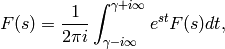
where  is chosen so that the contour path of
integration is in the region of convergence of .
is chosen so that the contour path of
integration is in the region of convergence of .
EXAMPLES:
sage: var('w, m')
(w, m)
sage: f = (1/(w^2+10)).inverse_laplace(w, m); f
1/10*sqrt(10)*sin(sqrt(10)*m)
sage: laplace(f, m, w)
1/(w^2 + 10)

sage: f(t) = t*cos(t)
sage: s = var('s')
sage: L = laplace(f, t, s); L
t |--> 2*s^2/(s^2 + 1)^2 - 1/(s^2 + 1)
sage: inverse_laplace(L, s, t)
t |--> t*cos(t)
sage: inverse_laplace(1/(s^3+1), s, t)
1/3*(sqrt(3)*sin(1/2*sqrt(3)*t) - cos(1/2*sqrt(3)*t))*e^(1/2*t) + 1/3*e^(-t)
No explicit inverse Laplace transform, so one is returned formally as a function ilt:
sage: inverse_laplace(cos(s), s, t)
ilt(cos(s), s, t)
Attempts to compute and return the Laplace transform of
self with respect to the variable and
transform parameter . If this function cannot find a
solution, a formal function is returned.
The function that is returned may be be viewed as a function of
.
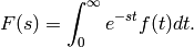
DEFINITION: The Laplace transform of a function ,
defined for all real numbers  , is the function
defined by
, is the function
defined by
EXAMPLES: We compute a few Laplace transforms:
sage: var('x, s, z, t, t0')
(x, s, z, t, t0)
sage: sin(x).laplace(x, s)
1/(s^2 + 1)
sage: (z + exp(x)).laplace(x, s)
z/s + 1/(s - 1)
sage: log(t/t0).laplace(t, s)
 -(euler_gamma + log(s) + log(t0))/s
We do a formal calculation:
sage: f = function('f', x)
sage: g = f.diff(x); g
D[0](f)(x)
sage: g.laplace(x, s)
s*laplace(f(x), x, s) - f(0)
EXAMPLE: A BATTLE BETWEEN the X-women and the Y-men (by David Joyner): Solve

This models a fight between two sides, the “X-women” and the “Y-men”, where the X-women have 270 initially and the Y-men have 90, but the Y-men are better at fighting, because of the higher factor of “-16” vs “-1”, and also get an occasional reinforcement, because of the “+1” term.
sage: var('t')
t
sage: t = var('t')
sage: x = function('x', t)
sage: y = function('y', t)
sage: de1 = x.diff(t) + 16*y
sage: de2 = y.diff(t) + x - 1
sage: de1.laplace(t, s)
s*laplace(x(t), t, s) + 16*laplace(y(t), t, s) - x(0)
sage: de2.laplace(t, s)
s*laplace(y(t), t, s) - 1/s + laplace(x(t), t, s) - y(0)
Next we form the augmented matrix of the above system:
sage: A = matrix([[s, 16, 270],[1, s, 90+1/s]])
sage: E = A.echelon_form()
sage: xt = E[0,2].inverse_laplace(s,t)
sage: yt = E[1,2].inverse_laplace(s,t)
sage: xt
629/2*e^(-4*t) - 91/2*e^(4*t) + 1
sage: yt
629/8*e^(-4*t) + 91/8*e^(4*t)
sage: p1 = plot(xt,0,1/2,rgbcolor=(1,0,0))
sage: p2 = plot(yt,0,1/2,rgbcolor=(0,1,0))
sage: (p1+p2).save(SAGE_TMP + "de_plot.png")
Another example:
sage: var('a,s,t')
(a, s, t)
sage: f = exp (2*t + a) * sin(t) * t; f
t*e^(a + 2*t)*sin(t)
sage: L = laplace(f, t, s); L
2*(s - 2)*e^a/(s^2 - 4*s + 5)^2
sage: inverse_laplace(L, s, t)
t*e^(a + 2*t)*sin(t)
Unable to compute solution:
sage: laplace(1/s, s, t)
laplace(1/s, s, t)
Return the limit as the variable  approaches
  from the given direction.
expr.limit(x = a)
expr.limit(x = a, dir='above')
INPUT:
Note
The output may also use ‘und’ (undefined), ‘ind’ (indefinite but bounded), and ‘infinity’ (complex infinity).
EXAMPLES:
sage: x = var('x')
sage: f = (1+1/x)^x
sage: f.limit(x = oo)
e
sage: f.limit(x = 5)
7776/3125
sage: f.limit(x = 1.2)
2.06961575467...
sage: f.limit(x = I, taylor=True)
(-I + 1)^I
sage: f(x=1.2)
2.0696157546720...
sage: f(x=I)
(-I + 1)^I
sage: CDF(f(x=I))
2.06287223508 + 0.74500706218*I
sage: CDF(f.limit(x = I))
2.06287223508 + 0.74500706218*I
More examples:
sage: limit(x*log(x), x = 0, dir='above')
0
sage: lim((x+1)^(1/x),x = 0)
e
sage: lim(e^x/x, x = oo)
+Infinity
sage: lim(e^x/x, x = -oo)
0
sage: lim(-e^x/x, x = oo)
-Infinity
sage: lim((cos(x))/(x^2), x = 0)
+Infinity
sage: lim(sqrt(x^2+1) - x, x = oo)
0
sage: lim(x^2/(sec(x)-1), x=0)
2
sage: lim(cos(x)/(cos(x)-1), x=0)
-Infinity
sage: lim(x*sin(1/x), x=0)
0
sage: f = log(log(x))/log(x)
sage: forget(); assume(x<-2); lim(f, x=0, taylor=True)
0
sage: forget()
Here ind means “indefinite but bounded”:
sage: lim(sin(1/x), x = 0)
ind
We check that Trac ticket 3718 is fixed, so that Maxima gives correct limits for the floor function:
sage: limit(floor(x),x=0,dir='below')
-1
sage: limit(floor(x),x=0,dir='above')
0
sage: limit(floor(x),x=0)
und
Maxima gives the right answer here, too, showing that Trac 4142 is fixed:
sage: f = sqrt(1-x^2)
sage: g = diff(f, x); g
-x/sqrt(-x^2 + 1)
sage: limit(g, x=1, dir='below')
-Infinity
TESTS:
sage: limit(1/x,x=0)
Infinity
sage: limit(1/x,x=0,dir='above')
+Infinity
sage: limit(1/x,x=0,dir='below')
-Infinity
Return the limit as the variable approaches
from the given direction.
expr.limit(x = a)
expr.limit(x = a, dir='above')
INPUT:
Note
The output may also use ‘und’ (undefined), ‘ind’ (indefinite but bounded), and ‘infinity’ (complex infinity).
EXAMPLES:
sage: x = var('x')
sage: f = (1+1/x)^x
sage: f.limit(x = oo)
e
sage: f.limit(x = 5)
7776/3125
sage: f.limit(x = 1.2)
2.06961575467...
sage: f.limit(x = I, taylor=True)
(-I + 1)^I
sage: f(x=1.2)
2.0696157546720...
sage: f(x=I)
(-I + 1)^I
sage: CDF(f(x=I))
2.06287223508 + 0.74500706218*I
sage: CDF(f.limit(x = I))
2.06287223508 + 0.74500706218*I
More examples:
sage: limit(x*log(x), x = 0, dir='above')
0
sage: lim((x+1)^(1/x),x = 0)
e
sage: lim(e^x/x, x = oo)
+Infinity
sage: lim(e^x/x, x = -oo)
0
sage: lim(-e^x/x, x = oo)
-Infinity
sage: lim((cos(x))/(x^2), x = 0)
+Infinity
sage: lim(sqrt(x^2+1) - x, x = oo)
0
sage: lim(x^2/(sec(x)-1), x=0)
2
sage: lim(cos(x)/(cos(x)-1), x=0)
-Infinity
sage: lim(x*sin(1/x), x=0)
0
sage: f = log(log(x))/log(x)
sage: forget(); assume(x<-2); lim(f, x=0, taylor=True)
0
sage: forget()
Here ind means “indefinite but bounded”:
sage: lim(sin(1/x), x = 0)
ind
We check that Trac ticket 3718 is fixed, so that Maxima gives correct limits for the floor function:
sage: limit(floor(x),x=0,dir='below')
-1
sage: limit(floor(x),x=0,dir='above')
0
sage: limit(floor(x),x=0)
und
Maxima gives the right answer here, too, showing that Trac 4142 is fixed:
sage: f = sqrt(1-x^2)
sage: g = diff(f, x); g
-x/sqrt(-x^2 + 1)
sage: limit(g, x=1, dir='below')
-Infinity
TESTS:
sage: limit(1/x,x=0)
Infinity
sage: limit(1/x,x=0,dir='above')
+Infinity
sage: limit(1/x,x=0,dir='below')
-Infinity
Used internally when creating a string of options to pass to Maxima.
INPUT:
OUTPUT: a string.
The main use of this is to turn Python bools into lower case strings.
EXAMPLES:
sage: sage.calculus.calculus.mapped_opts(True)
'true'
sage: sage.calculus.calculus.mapped_opts(False)
'false'
sage: sage.calculus.calculus.mapped_opts('bar')
'bar'
Used internally to create a string of options to pass to Maxima.
EXAMPLES:
sage: sage.calculus.calculus.maxima_options(an_option=True, another=False, foo='bar')
'an_option=true,foo=bar,another=false'
Return the minimal polynomial of self, if possible.
INPUT:
var - polynomial variable name (default ‘x’)
algorithm - ‘algebraic’ or ‘numerical’ (default both, but with numerical first)
bits - the number of bits to use in numerical approx
degree - the expected algebraic degree
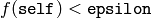
epsilon - return without error as long as f(self) epsilon, in the case that the result cannot be proven.
All of the above parameters are optional, with epsilon=0, bits and degree tested up to 1000 and 24 by default respectively. The numerical algorithm will be faster if bits and/or degree are given explicitly. The algebraic algorithm ignores the last three parameters.
OUTPUT: The minimal polynomial of self. If the numerical algorithm is used then it is proved symbolically when epsilon=0 (default).
If the minimal polynomial could not be found, two distinct kinds of errors are raised. If no reasonable candidate was found with the given bit/degree parameters, a ValueError will be raised. If a reasonable candidate was found but (perhaps due to limits in the underlying symbolic package) was unable to be proved correct, a NotImplementedError will be raised.
ALGORITHM: Two distinct algorithms are used, depending on the algorithm parameter. By default, the numerical algorithm is attempted first, then the algebraic one.
Algebraic: Attempt to evaluate this expression in QQbar, using cyclotomic fields to resolve exponential and trig functions at rational multiples of pi, field extensions to handle roots and rational exponents, and computing compositums to represent the full expression as an element of a number field where the minimal polynomial can be computed exactly. The bits, degree, and epsilon parameters are ignored.
Numerical: Computes a numerical approximation of
self and use PARI’s algdep to get a candidate
minpoly  . If
. If  ,
evaluated to a higher precision, is close enough to 0 then evaluate
symbolically, attempting to prove
vanishing. If this fails, and epsilon is non-zero,
return if and only if
,
evaluated to a higher precision, is close enough to 0 then evaluate
symbolically, attempting to prove
vanishing. If this fails, and epsilon is non-zero,
return if and only if
 .
Otherwise raise a ValueError (if no suitable
candidate was found) or a NotImplementedError (if a
likely candidate was found but could not be proved correct).
.
Otherwise raise a ValueError (if no suitable
candidate was found) or a NotImplementedError (if a
likely candidate was found but could not be proved correct).
EXAMPLES: First some simple examples:
sage: sqrt(2).minpoly()
x^2 - 2
sage: minpoly(2^(1/3))
x^3 - 2
sage: minpoly(sqrt(2) + sqrt(-1))
x^4 - 2*x^2 + 9
sage: minpoly(sqrt(2)-3^(1/3))
x^6 - 6*x^4 + 6*x^3 + 12*x^2 + 36*x + 1
Works with trig and exponential functions too.
sage: sin(pi/3).minpoly()
x^2 - 3/4
sage: sin(pi/7).minpoly()
x^6 - 7/4*x^4 + 7/8*x^2 - 7/64
sage: minpoly(exp(I*pi/17))
x^16 - x^15 + x^14 - x^13 + x^12 - x^11 + x^10 - x^9 + x^8 - x^7 + x^6 - x^5 + x^4 - x^3 + x^2 - x + 1
Here we verify it gives the same result as the abstract number field.
sage: (sqrt(2) + sqrt(3) + sqrt(6)).minpoly()
x^4 - 22*x^2 - 48*x - 23
sage: K.<a,b> = NumberField([x^2-2, x^2-3])
sage: (a+b+a*b).absolute_minpoly()
x^4 - 22*x^2 - 48*x - 23
The minpoly function is used implicitly when creating number fields:
sage: x = var('x')
sage: eqn =  x^3 + sqrt(2)*x + 5 == 0
sage: a = solve(eqn, x)[0].rhs()
sage: QQ[a]
Number Field in a with defining polynomial x^6 + 10*x^3 - 2*x^2 + 25
Here we solve a cubic and then recover it from its complicated radical expansion.
sage: f = x^3 - x + 1
sage: a = f.solve(x)[0].rhs(); a
-1/2*(I*sqrt(3) + 1)*(1/18*sqrt(3)*sqrt(23) - 1/2)^(1/3) - 1/6*(-I*sqrt(3) + 1)/(1/18*sqrt(3)*sqrt(23) - 1/2)^(1/3)
sage: a.minpoly()
x^3 - x + 1
Note that simplification may be necessary to see that the minimal polynomial is correct.
sage: a = sqrt(2)+sqrt(3)+sqrt(5)
sage: f = a.minpoly(); f
x^8 - 40*x^6 + 352*x^4 - 960*x^2 + 576
sage: f(a)
((((sqrt(2) + sqrt(3) + sqrt(5))^2 - 40)*(sqrt(2) + sqrt(3) + sqrt(5))^2 + 352)*(sqrt(2) + sqrt(3) + sqrt(5))^2 - 960)*(sqrt(2) + sqrt(3) + sqrt(5))^2 + 576
sage: f(a).expand()
0
Here we show use of the epsilon parameter. That this result is actually exact can be shown using the addition formula for sin, but maxima is unable to see that.
sage: a = sin(pi/5)
sage: a.minpoly(algorithm='numerical')
...
NotImplementedError: Could not prove minimal polynomial x^4 - 5/4*x^2 + 5/16 (epsilon 0.00000000000000e-1)
sage: f = a.minpoly(algorithm='numerical', epsilon=1e-100); f
x^4 - 5/4*x^2 + 5/16
sage: f(a).numerical_approx(100)
0.00000000000000000000000000000
The degree must be high enough (default tops out at 24).
sage: a = sqrt(3) + sqrt(2)
sage: a.minpoly(algorithm='numerical', bits=100, degree=3)
...
ValueError: Could not find minimal polynomial (100 bits, degree 3).
sage: a.minpoly(algorithm='numerical', bits=100, degree=10)
x^4 - 10*x^2 + 1
There is a difference between algorithm=’algebraic’ and algorithm=’numerical’:
sage: cos(pi/33).minpoly(algorithm='algebraic')
x^10 + 1/2*x^9 - 5/2*x^8 - 5/4*x^7 + 17/8*x^6 + 17/16*x^5 - 43/64*x^4 - 43/128*x^3 + 3/64*x^2 + 3/128*x + 1/1024
sage: cos(pi/33).minpoly(algorithm='numerical')
...
NotImplementedError: Could not prove minimal polynomial x^10 + 1/2*x^9 - 5/2*x^8 - 5/4*x^7 + 17/8*x^6 + 17/16*x^5 - 43/64*x^4 - 43/128*x^3 + 3/64*x^2 + 3/128*x + 1/1024 (epsilon ...)
Sometimes it fails, as it must given that some numbers aren’t algebraic:
sage: sin(1).minpoly(algorithm='numerical')
...
ValueError: Could not find minimal polynomial (1000 bits, degree 24).
Note
Of course, failure to produce a minimal polynomial does not necessarily indicate that this number is transcendental.
Return a floating point machine precision numerical approximation
to the integral of self from to
 , computed using floating point arithmetic via maxima.
INPUT:
OUTPUT:
ALIAS: nintegrate is the same as nintegral
REMARK: There is also a function numerical_integral that implements numerical integration using the GSL C library. It is potentially much faster and applies to arbitrary user defined functions.
Also, there are limits to the precision to which Maxima can compute the integral to due to limitations in quadpack.
sage: f = x
sage: f = f.nintegral(x,0,1,1e-14)
...
ValueError: Maxima (via quadpack) cannot compute the integral to that precision
EXAMPLES:
sage: f(x) = exp(-sqrt(x))
sage: f.nintegral(x, 0, 1)
(0.52848223531423055, 4.163...e-11, 231, 0)
We can also use the numerical_integral function, which calls the GSL C library.
sage: numerical_integral(f, 0, 1)
(0.52848223225314706, 6.83928460...e-07)
Note that in exotic cases where floating point evaluation of the expression leads to the wrong value, then the output can be completely wrong:
sage: f = exp(pi*sqrt(163)) - 262537412640768744
Despite appearance, is really very close to 0, but one
gets a nonzero value since the definition of
float(f) is that it makes all constants inside the
expression floats, then evaluates each function and each arithmetic
operation using float arithmetic:
sage: float(f)
-480.0
Computing to higher precision we see the truth:
sage: f.n(200)
-7.4992740280181431112064614366622348652078895136533593355718e-13
sage: f.n(300)
-7.49927402801814311120646143662663009137292462589621789352095066181709095575681963967103004e-13
Now numerically integrating, we see why the answer is wrong:
sage: f.nintegrate(x,0,1)
(-480.00000000000011, 5.3290705182007538e-12, 21, 0)
It is just because every floating point evaluation of return -480.0 in floating point.
Important note: using GP/PARI one can compute numerical integrals to high precision:
sage: gp.eval('intnum(x=17,42,exp(-x^2)*log(x))')
'2.565728500561051482917356396 E-127'        # 32-bit
'2.5657285005610514829173563961304785900 E-127'    # 64-bit
sage: old_prec = gp.set_real_precision(50)
sage: gp.eval('intnum(x=17,42,exp(-x^2)*log(x))')
'2.5657285005610514829173563961304785900147709554020 E-127'
sage: gp.set_real_precision(old_prec)
57
Note that the input function above is a string in PARI syntax.
Return a floating point machine precision numerical approximation
to the integral of self from to
, computed using floating point arithmetic via maxima.
INPUT:
OUTPUT:
ALIAS: nintegrate is the same as nintegral
REMARK: There is also a function numerical_integral that implements numerical integration using the GSL C library. It is potentially much faster and applies to arbitrary user defined functions.
Also, there are limits to the precision to which Maxima can compute the integral to due to limitations in quadpack.
sage: f = x
sage: f = f.nintegral(x,0,1,1e-14)
...
ValueError: Maxima (via quadpack) cannot compute the integral to that precision
EXAMPLES:
sage: f(x) = exp(-sqrt(x))
sage: f.nintegral(x, 0, 1)
(0.52848223531423055, 4.163...e-11, 231, 0)
We can also use the numerical_integral function, which calls the GSL C library.
sage: numerical_integral(f, 0, 1)
(0.52848223225314706, 6.83928460...e-07)
Note that in exotic cases where floating point evaluation of the expression leads to the wrong value, then the output can be completely wrong:
sage: f = exp(pi*sqrt(163)) - 262537412640768744
Despite appearance, is really very close to 0, but one
gets a nonzero value since the definition of
float(f) is that it makes all constants inside the
expression floats, then evaluates each function and each arithmetic
operation using float arithmetic:
sage: float(f)
-480.0
Computing to higher precision we see the truth:
sage: f.n(200)
-7.4992740280181431112064614366622348652078895136533593355718e-13
sage: f.n(300)
-7.49927402801814311120646143662663009137292462589621789352095066181709095575681963967103004e-13
Now numerically integrating, we see why the answer is wrong:
sage: f.nintegrate(x,0,1)
(-480.00000000000011, 5.3290705182007538e-12, 21, 0)
It is just because every floating point evaluation of return -480.0 in floating point.
Important note: using GP/PARI one can compute numerical integrals to high precision:
sage: gp.eval('intnum(x=17,42,exp(-x^2)*log(x))')
'2.565728500561051482917356396 E-127'        # 32-bit
'2.5657285005610514829173563961304785900 E-127'    # 64-bit
sage: old_prec = gp.set_real_precision(50)
sage: gp.eval('intnum(x=17,42,exp(-x^2)*log(x))')
'2.5657285005610514829173563961304785900147709554020 E-127'
sage: gp.set_real_precision(old_prec)
57
Note that the input function above is a string in PARI syntax.
Given a string representation of a Maxima expression, parse it and return the corresponding Sage symbolic expression.
INPUT:
EXAMPLES:
sage: from sage.calculus.calculus import symbolic_expression_from_maxima_string as sefms
sage: sefms('x^%e + %e^%pi + %i + sin(0)')
x^e + e^pi + I
sage: f = function('f',x)
sage: sefms('?%at(f(x),x=2)#1')
f(2) != 1
sage: a = sage.calculus.calculus.maxima("x#0"); a
x#0
sage: a.sage()
x != 0
TESTS:
Trac #8459 fixed:
sage: maxima('3*li[2](u)+8*li[33](exp(u))').sage()
3*polylog(2, u) + 8*polylog(33, e^u)
Given a string, (attempt to) parse it and return the corresponding Sage symbolic expression. Normally used to return Maxima output to the user.
INPUT:
EXAMPLES:
sage: y = var('y')
sage: sage.calculus.calculus.symbolic_expression_from_string('[sin(0)*x^2,3*spam+e^pi]',syms={'spam':y},accept_sequence=True)
[0, 3*y + e^pi]
Returns the symbolic sum 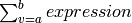 with respect
to the variable with endpoints and .
with respect
to the variable with endpoints and .
INPUT:
EXAMPLES:
sage: k, n = var('k,n')
sage: from sage.calculus.calculus import symbolic_sum
sage: symbolic_sum(k, k, 1, n).factor()
1/2*(n + 1)*n
sage: symbolic_sum(1/k^4, k, 1, oo)
1/90*pi^4
sage: symbolic_sum(1/k^5, k, 1, oo)
zeta(5)
A well known binomial identity:
sage: symbolic_sum(binomial(n,k), k, 0, n)
2^n
And some truncations thereof:
sage: symbolic_sum(binomial(n,k),k,1,n)
2^n - 1
sage: symbolic_sum(binomial(n,k),k,2,n)
2^n - n - 1
sage: symbolic_sum(binomial(n,k),k,0,n-1)
2^n - 1
sage: symbolic_sum(binomial(n,k),k,1,n-1)
2^n - 2
The binomial theorem:
sage: x, y = var('x, y')
sage: symbolic_sum(binomial(n,k) * x^k * y^(n-k), k, 0, n)
(x + y)^n
sage: symbolic_sum(k * binomial(n, k), k, 1, n)
n*2^(n - 1)
sage: symbolic_sum((-1)^k*binomial(n,k), k, 0, n)
0
sage: symbolic_sum(2^(-k)/(k*(k+1)), k, 1, oo)
-log(2) + 1
Summing a hypergeometric term:
sage: symbolic_sum(binomial(n, k) * factorial(k) / factorial(n+1+k), k, 0, n)
1/2*sqrt(pi)/factorial(n + 1/2)
We check a well known identity:
sage: bool(symbolic_sum(k^3, k, 1, n) == symbolic_sum(k, k, 1, n)^2)
True
A geometric sum:
sage: a, q = var('a, q')
sage: symbolic_sum(a*q^k, k, 0, n)
(a*q^(n + 1) - a)/(q - 1)
The geometric series:
sage: assume(abs(q) < 1)
sage: symbolic_sum(a*q^k, k, 0, oo)
-a/(q - 1)
A divergent geometric series. Don’t forget to forget your assumptions:
sage: forget()
sage: assume(q > 1)
sage: symbolic_sum(a*q^k, k, 0, oo)
...
ValueError: Sum is divergent.
This summation only Mathematica can perform:
sage: symbolic_sum(1/(1+k^2), k, -oo, oo, algorithm = 'mathematica')     # optional  -- requires mathematica
pi*coth(pi)
Use Maple as a backend for summation:
sage: symbolic_sum(binomial(n,k)*x^k, k, 0, n, algorithm = 'maple')      # optional  -- requires maple
(x + 1)^n
Note
Return comparison of the two variables x and y, which is just the comparison of the underlying string representations of the variables. This is used internally by the Calculus package.
INPUT:
OUTPUT: Python integer; either -1, 0, or 1.
EXAMPLES:
sage: sage.calculus.calculus.var_cmp(x,x)
0
sage: sage.calculus.calculus.var_cmp(x,var('z'))
-1
sage: sage.calculus.calculus.var_cmp(x,var('a'))
1
