Modular parametrization of elliptic curves over .

By the work of Talyor-Wiles et al. it is known that there is a surjective morphism

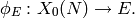
from the modular curve , where is the conductor of . The map sends the cusp to the origin of .

EXMAPLES:

sage: phi = EllipticCurve('11a1').modular_parametrization()
sage: phi
Modular parameterization from the upper half plane to Elliptic Curve defined by y^2 + y = x^3 - x^2 - 10*x - 20 over Rational Field
sage: phi(0.5+CDF(I))
(285684.320516... + 7.01033491...e-11*I : 1.526964169...e8 + 5.6214048527...e-8*I : 1.00000000000000)
sage: phi.power_series()
(q^-2 + 2*q^-1 + 4 + 5*q + 8*q^2 + q^3 + 7*q^4 - 11*q^5 + 10*q^6 - 12*q^7 - 18*q^8 - 22*q^9 + 26*q^10 - 11*q^11 + 41*q^12 + 44*q^13 - 15*q^14 + 19746*q^15 + 51565*q^16 + 150132*q^17 + O(q^18), -q^-3 - 3*q^-2 - 7*q^-1 - 13 - 17*q - 26*q^2 - 19*q^3 - 37*q^4 + 15*q^5 + 16*q^6 + 67*q^7 + 6*q^8 + 144*q^9 - 92*q^10 + 66*q^11 - 119*q^12 - 95*q^13 + 176205*q^14 + 669718*q^15 + 2562150*q^16 + O(q^17))

AUTHORS:

• chris wuthrich (02/10) - moved from ell_rational_field.py.

class sage.schemes.elliptic_curves.modular_parametrization.ModularParameterization(E)

This class represents the modular parametrization of an elliptic curve

Evaluation is done by passing through the lattice representation of .

EXAMPLES:

sage: phi = EllipticCurve('11a1').modular_parametrization()
sage: phi
Modular parameterization from the upper half plane to Elliptic Curve defined by y^2 + y = x^3 - x^2 - 10*x - 20 over Rational Field

curve()

Returns the curve associated to this modular parametrization.

EXAMPLES:

sage: E = EllipticCurve('15a')
sage: phi = E.modular_parametrization()
sage: phi.curve() is E
True

map_to_complex_numbers(z, prec=None)

Evaluate self at a point where is given by a representative in the upper half plane, returning a point in the complex numbers. All computations done with prec bits of precision. If prec is not given, use the precision of . Use self(z) to compute the image of z on the Weierstrass equation of the curve.

EXAMPLES:

sage: E = EllipticCurve('37a'); phi = E.modular_parametrization()
sage: tau = (sqrt(7)*I - 17)/74
sage: z = phi.map_to_complex_numbers(tau); z
0.929592715285395 - 1.22569469099340*I
sage: E.elliptic_exponential(z)
(...e-16 - ...e-16*I : ...e-16 + ...e-16*I : 1.00000000000000)
sage: phi(tau)
(...e-16 - ...e-16*I : ...e-16 + ...e-16*I : 1.00000000000000)            

power_series()

Computes and returns the power series of this modular parametrization.

The curve must be a a minimal model.

OUTPUT: A list of two Laurent series [X(x),Y(x)] of degrees -2, -3 respectively, which satisfy the equation of the elliptic curve. There are modular functions on where is the conductor.

The series should satisfy the differential equation

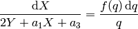
where is self.curve().q_expansion().

EXAMPLES:

sage: E=EllipticCurve('389a1')
sage: phi = E.modular_parametrization()
sage: X,Y = phi.power_series()
sage: X
q^-2 + 2*q^-1 + 4 + 7*q + 13*q^2 + 18*q^3 + 31*q^4 + 49*q^5 + 74*q^6 + 111*q^7 + 173*q^8 + 251*q^9 + 379*q^10 + 560*q^11 + 824*q^12 + 1199*q^13 + 1773*q^14 + 2365*q^15 + 3463*q^16 + 4508*q^17 + O(q^18)
sage: Y
-q^-3 - 3*q^-2 - 8*q^-1 - 17 - 33*q - 61*q^2 - 110*q^3 - 186*q^4 - 320*q^5 - 528*q^6 - 861*q^7 - 1383*q^8 - 2218*q^9 - 3472*q^10 - 5451*q^11 - 8447*q^12 - 13020*q^13 - 20083*q^14 - 29512*q^15 - 39682*q^16 + O(q^17)

The following should give 0, but only approximately:

sage: q = X.parent().gen()
sage: E.defining_polynomial()(X,Y,1) + O(q^11) == 0
True

Note that below we have to change variable from x to q:

sage: a1,_,a3,_,_=E.a_invariants()
sage: f=E.q_expansion(17)
sage: q=f.parent().gen()
sage: f/q == (X.derivative()/(2*Y+a1*X+a3))
True