Elliptic curves over the rational numbers¶

AUTHORS:

William Stein (2005): first version
William Stein (2006-02-26): fixed Lseries_extended which didn’t work because of changes elsewhere in Sage.
David Harvey (2006-09): Added padic_E2, padic_sigma, padic_height, padic_regulator methods.
David Harvey (2007-02): reworked padic-height related code
Christian Wuthrich (2007): added padic sha computation
David Roe (2007-09): moved sha, l-series and p-adic functionality to separate files.
John Cremona (2008-01)
Tobias Nagel and Michael Mardaus (2008-07): added integral_points
John Cremona (2008-07): further work on integral_points
Christian Wuthrich (2010-01): moved Galois reps and modular parametrization in a separate file

class sage.schemes.elliptic_curves.ell_rational_field.EllipticCurve_rational_field(ainvs, extra=None)¶

Bases: sage.schemes.elliptic_curves.ell_number_field.EllipticCurve_number_field

Elliptic curve over the Rational Field.

INPUT:

ainvs (list or string) – either $[a_1,a_2,a_3,a_4,a_6]$ or $[a_4,a_6]$ (with $a_1=a_2=a_3=0$ ) or a valid label from the database.

Note

See constructor.py for more variants.

EXAMPLES:

Construction from Weierstrass coefficients ( $a$ -invariants), long form:

sage: E = EllipticCurve([1,2,3,4,5]); E
Elliptic Curve defined by y^2 + x*y + 3*y = x^3 + 2*x^2 + 4*x + 5 over Rational Field

Construction from Weierstrass coefficients ( $a$ -invariants), short form (sets $a_1=a_2=a_3=0$ ):

sage: EllipticCurve([4,5]).ainvs()
(0, 0, 0, 4, 5)

Construction from a database label:

sage: EllipticCurve('389a1')
Elliptic Curve defined by y^2 + y = x^3 + x^2 - 2*x over Rational Field

CPS_height_bound()¶

Return the Cremona-Prickett-Siksek height bound. This is a floating point number B such that if P is a rational point on the curve, then 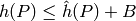$h(P) \le \hat{h}(P) + B$ , where $h(P)$ is the naive logarithmic height of $P$ and $\hat{h}(P)$ is the canonical height.

SEE ALSO: silverman_height_bound for a bound that also works for points over number fields.

EXAMPLES:

sage: E = EllipticCurve("11a")
sage: E.CPS_height_bound()
2.8774743273580445
sage: E = EllipticCurve("5077a")
sage: E.CPS_height_bound()
0.0
sage: E = EllipticCurve([1,2,3,4,1])
sage: E.CPS_height_bound()
...
RuntimeError: curve must be minimal.
sage: F = E.quadratic_twist(-19)
sage: F
Elliptic Curve defined by y^2 + x*y + y = x^3 - x^2 + 1376*x - 130 over Rational Field
sage: F.CPS_height_bound()
0.65551583769728516

IMPLEMENTATION:: Call the corresponding mwrank C++ library function. Note that the formula in the [CPS] paper is given for number fields. It’s only the implementation in Sage that restricts to the rational field.

Lambda(s, prec)¶

Returns the value of the Lambda-series of the elliptic curve E at s, where s can be any complex number.

IMPLEMENTATION: Fairly slow computation using the definitions and implemented in Python.

Uses prec terms of the power series.

EXAMPLES:

sage: E = EllipticCurve('389a')
sage: E.Lambda(1.4+0.5*I, 50)
-0.354172680517... + 0.874518681720...*I

Np(p)¶

The number of points on $E$ modulo $p$ .

INPUT:

p (int) – a prime, not necessarily of good reduction.

OUTPUT:

(int) The number ofpoints on the reduction of $E$ modulo $p$ (including the singular point when $p$ is a prime of bad reduction).

EXAMPLES:

sage: E = EllipticCurve([0, -1, 1, -10, -20])
sage: E.Np(2)
5
sage: E.Np(3)
5
sage: E.conductor()
11
sage: E.Np(11)
11

S_integral_points(S, mw_base='auto', both_signs=False, verbose=False, proof=None)¶

Computes all S-integral points (up to sign) on this elliptic curve.

INPUT:

S - list of primes
mw_base - list of EllipticCurvePoint generating the Mordell-Weil group of E (default: ‘auto’ - calls gens())
both_signs - True/False (default False): if True the output contains both P and -P, otherwise only one of each pair.
verbose - True/False (default False): if True, some details of the computation are output.
proof - True/False (default True): if True ALL S-integral points will be returned. If False, the MW basis will be computed with the proof=False flag, and also the time-consuming final call to S_integral_x_coords_with_abs_bounded_by(abs_bound) is omitted. Use this only if the computation takes too long, but be warned that then it cannot be guaranteed that all S-integral points will be found.

OUTPUT:

A sorted list of all the S-integral points on E (up to sign unless both_signs is True)

Note

The complexity increases exponentially in the rank of curve E and in the length of S. The computation time (but not the output!) depends on the Mordell-Weil basis. If mw_base is given but is not a basis for the Mordell-Weil group (modulo torsion), S-integral points which are not in the subgroup generated by the given points will almost certainly not be listed.

EXAMPLES:

A curve of rank 3 with no torsion points:

sage: E=EllipticCurve([0,0,1,-7,6])
sage: P1=E.point((2,0)); P2=E.point((-1,3)); P3=E.point((4,6))
sage: a=E.S_integral_points(S=[2,3], mw_base=[P1,P2,P3], verbose=True);a
max_S: 3 len_S: 3 len_tors: 1
lambda 0.485997517468...
k1,k2,k3,k4 6.68597129142710e234 1.31952866480763 3.31908110593519e9 2.42767548272846e17
p= 2 : trying with p_prec =  30
mw_base_p_log_val =  [2, 2, 1]
min_psi =  2 + 2^3 + 2^6 + 2^7 + 2^8 + 2^9 + 2^11 + 2^12 + 2^13 + 2^16 + 2^17 + 2^19 + 2^20 + 2^21 + 2^23 + 2^24 + 2^28 + O(2^30)
p= 3 : trying with p_prec =  30
mw_base_p_log_val =  [1, 2, 1]
min_psi =  3 + 3^2 + 2*3^3 + 3^6 + 2*3^7 + 2*3^8 + 3^9 + 2*3^11 + 2*3^12 + 2*3^13 + 3^15 + 2*3^16 + 3^18 + 2*3^19 + 2*3^22 + 2*3^23 + 2*3^24 + 2*3^27 + 3^28 + 3^29 + O(3^30)
mw_base [(1 : -1 : 1), (2 : 0 : 1), (0 : -3 : 1)]
mw_base_log [0.667789378224099, 0.552642660712417, 0.818477222895703]
mp [5, 7]
mw_base_p_log [[2^2 + 2^3 + 2^6 + 2^7 + 2^8 + 2^9 + 2^14 + 2^15 + 2^18 + 2^19 + 2^24 + 2^29 + O(2^30), 2^2 + 2^3 + 2^5 + 2^6 + 2^9 + 2^11 + 2^12 + 2^14 + 2^15 + 2^16 + 2^18 + 2^20 + 2^22 + 2^23 + 2^26 + 2^27 + 2^29 + O(2^30), 2 + 2^3 + 2^6 + 2^7 + 2^8 + 2^9 + 2^11 + 2^12 + 2^13 + 2^16 + 2^17 + 2^19 + 2^20 + 2^21 + 2^23 + 2^24 + 2^28 + O(2^30)], [2*3^2 + 2*3^5 + 2*3^6 + 2*3^7 + 3^8 + 3^9 + 2*3^10 + 3^12 + 2*3^14 + 3^15 + 3^17 + 2*3^19 + 2*3^23 + 3^25 + 3^28 + O(3^30), 2*3 + 2*3^2 + 2*3^3 + 2*3^4 + 2*3^6 + 2*3^7 + 2*3^8 + 3^10 + 2*3^12 + 3^13 + 2*3^14 + 3^15 + 3^18 + 3^22 + 3^25 + 2*3^26 + 3^27 + 3^28 + O(3^30), 3 + 3^2 + 2*3^3 + 3^6 + 2*3^7 + 2*3^8 + 3^9 + 2*3^11 + 2*3^12 + 2*3^13 + 3^15 + 2*3^16 + 3^18 + 2*3^19 + 2*3^22 + 2*3^23 + 2*3^24 + 2*3^27 + 3^28 + 3^29 + O(3^30)]]
k5,k6,k7 0.321154513240... 1.55246328915... 0.161999172489...
initial bound 2.6227097483365...e117
bound_list [58, 58, 58]
bound_list [8, 9, 9]
bound_list [8, 7, 7]
bound_list [8, 7, 7]
starting search of points using coefficient bound  8
x-coords of S-integral points via linear combination of mw_base and torsion:
[-3, -26/9, -8159/2916, -2759/1024, -151/64, -1343/576, -2, -7/4, -1, -47/256, 0, 1/4, 4/9, 9/16, 58/81, 7/9, 6169/6561, 1, 17/16, 2, 33/16, 172/81, 9/4, 25/9, 3, 31/9, 4, 25/4, 1793/256, 8, 625/64, 11, 14, 21, 37, 52, 6142/81, 93, 4537/36, 342, 406, 816, 207331217/4096]
starting search of extra S-integer points with absolute value bounded by 3.89321964979420
x-coords of points with bounded absolute value
[-3, -2, -1, 0, 1, 2]
Total number of S-integral points: 43
[(-3 : 0 : 1), (-26/9 : 28/27 : 1), (-8159/2916 : 233461/157464 : 1), (-2759/1024 : 60819/32768 : 1), (-151/64 : 1333/512 : 1), (-1343/576 : 36575/13824 : 1), (-2 : 3 : 1), (-7/4 : 25/8 : 1), (-1 : 3 : 1), (-47/256 : 9191/4096 : 1), (0 : 2 : 1), (1/4 : 13/8 : 1), (4/9 : 35/27 : 1), (9/16 : 69/64 : 1), (58/81 : 559/729 : 1), (7/9 : 17/27 : 1), (6169/6561 : 109871/531441 : 1), (1 : 0 : 1), (17/16 : -25/64 : 1), (2 : 0 : 1), (33/16 : 17/64 : 1), (172/81 : 350/729 : 1), (9/4 : 7/8 : 1), (25/9 : 64/27 : 1), (3 : 3 : 1), (31/9 : 116/27 : 1), (4 : 6 : 1), (25/4 : 111/8 : 1), (1793/256 : 68991/4096 : 1), (8 : 21 : 1), (625/64 : 14839/512 : 1), (11 : 35 : 1), (14 : 51 : 1), (21 : 95 : 1), (37 : 224 : 1), (52 : 374 : 1), (6142/81 : 480700/729 : 1), (93 : 896 : 1), (4537/36 : 305425/216 : 1), (342 : 6324 : 1), (406 : 8180 : 1), (816 : 23309 : 1), (207331217/4096 : 2985362173625/262144 : 1)]

It is not necessary to specify mw_base; if it is not provided, then the Mordell-Weil basis must be computed, which may take much longer.

sage: a = E.S_integral_points([2,3])
sage: len(a)
43

An example with negative discriminant:

sage: EllipticCurve('900d1').S_integral_points([17], both_signs=True) 
[(-11 : -27 : 1), (-11 : 27 : 1), (-4 : -34 : 1), (-4 : 34 : 1), (4 : -18 : 1), (4 : 18 : 1), (2636/289 : -98786/4913 : 1), (2636/289 : 98786/4913 : 1), (16 : -54 : 1), (16 : 54 : 1)]

Output checked with Magma (corrected in 3 cases):

sage: [len(e.S_integral_points([2], both_signs=False)) for e in cremona_curves([11..100])] # long time
[2, 0, 2, 3, 3, 1, 3, 1, 3, 5, 3, 5, 4, 1, 1, 2, 2, 2, 3, 1, 2, 1, 0, 1, 3, 3, 1, 1, 5, 3, 4, 2, 1, 1, 5, 3, 2, 2, 1, 1, 1, 0, 1, 3, 0, 1, 0, 1, 1, 3, 7, 1, 3, 3, 3, 1, 1, 2, 3, 1, 2, 3, 1, 2, 1, 3, 3, 1, 1, 1, 0, 1, 3, 3, 1, 1, 7, 1, 0, 1, 1, 0, 1, 2, 0, 3, 1, 2, 1, 3, 1, 2, 2, 4, 5, 3, 2, 1, 1, 6, 1, 0, 1, 3, 1, 3, 3, 1, 1, 1, 1, 1, 3, 1, 5, 1, 2, 4, 1, 1, 1, 1, 1, 0, 1, 0, 2, 2, 0, 0, 1, 0, 1, 1, 6, 1, 0, 1, 1, 0, 4, 3, 1, 2, 1, 2, 3, 1, 1, 1, 1, 8, 3, 1, 2, 1, 2, 0, 8, 2, 0, 6, 2, 3, 1, 1, 1, 3, 1, 3, 2, 1, 3, 1, 2, 1, 6, 9, 3, 3, 1, 1, 2, 3, 1, 1, 5, 5, 1, 1, 0, 1, 1, 2, 3, 1, 1, 2, 3, 1, 3, 1, 1, 1, 1, 0, 0, 1, 3, 3, 1, 3, 1, 1, 2, 2, 0, 0, 6, 1, 0, 1, 1, 1, 1, 3, 1, 2, 6, 3, 1, 2, 2, 1, 1, 1, 1, 7, 5, 4, 3, 3, 1, 1, 1, 1, 1, 1, 8, 5, 1, 1, 3, 3, 1, 1, 3, 3, 1, 1, 2, 3, 6, 1, 1, 7, 3, 3, 4, 5, 9, 6, 1, 0, 7, 1, 1, 3, 1, 1, 2, 3, 1, 2, 1, 1, 1, 1, 1, 1, 1, 7, 8, 2, 3, 1, 1, 1, 1, 0, 0, 0, 1, 1, 1, 1]

An example from [PZGH]:

sage: E = EllipticCurve([0,0,0,-172,505])
sage: E.rank(), len(E.S_integral_points([3,5,7]))  # long time (~7s)
(4, 72)

This is curve “7690e1” which failed until #4805 was fixed:

sage: EllipticCurve([1,1,1,-301,-1821]).S_integral_points([13,2])
[(-13 : 16 : 1),
(-9 : 20 : 1),
(-7 : 4 : 1),
(21 : 30 : 1),
(23 : 52 : 1),
(63 : 452 : 1),
(71 : 548 : 1),
(87 : 756 : 1),
(2711 : 139828 : 1),
(7323 : 623052 : 1),
(17687 : 2343476 : 1)]

REFERENCES:

[PZGH] Petho A., Zimmer H.G., Gebel J. and Herrmann E., Computing all S-integral points on elliptic curves Math. Proc. Camb. Phil. Soc. (1999), 127, 383-402
Some parts of this implementation are partially based on the function integral_points()

AUTHORS:

Tobias Nagel (2008-12)
Michael Mardaus (2008-12)
John Cremona (2008-12)

an(n)¶

The n-th Fourier coefficient of the modular form corresponding to this elliptic curve, where n is a positive integer.

EXAMPLES:

sage: E=EllipticCurve('37a1')
sage: [E.an(n) for n in range(20) if n>0]
[1, -2, -3, 2, -2, 6, -1, 0, 6, 4, -5, -6, -2, 2, 6, -4, 0, -12, 0]

analytic_rank(algorithm='cremona')¶

Return an integer that is probably the analytic rank of this elliptic curve.

INPUT:

algorithm -
- ‘cremona’ (default) - Use the Buhler-Gross algorithm as implemented in GP by Tom Womack and John Cremona, who note that their implementation is practical for any rank and conductor $\leq 10^{10}$ in 10 minutes.
- ‘sympow’ -use Watkins’s program sympow
- ‘rubinstein’ - use Rubinstein’s L-function C++ program lcalc.
- ‘magma’ - use MAGMA
- ‘all’ - compute with all other free algorithms, check that the answers agree, and return the common answer.

Note

If the curve is loaded from the large Cremona database, then the modular degree is taken from the database.

Of the three above, probably Rubinstein’s is the most efficient (in some limited testing I’ve done).

Note

It is an open problem to prove that any particular elliptic curve has analytic rank $\geq 4$ .

EXAMPLES:

sage: E = EllipticCurve('389a')
sage: E.analytic_rank(algorithm='cremona')
2
sage: E.analytic_rank(algorithm='rubinstein')
2
sage: E.analytic_rank(algorithm='sympow')
2
sage: E.analytic_rank(algorithm='magma')    # optional - magma
2
sage: E.analytic_rank(algorithm='all')
2

TESTS:

When the input is horrendous, some of the algorithms just bomb out with a RuntimeError:

sage: EllipticCurve([1234567,89101112]).analytic_rank(algorithm='rubinstein')
...
RuntimeError: unable to compute analytic rank using rubinstein algorithm ('unable to convert x (= 6.19283e+19 and is too large) to an integer')
sage: EllipticCurve([1234567,89101112]).analytic_rank(algorithm='sympow')
...
RuntimeError: failed to compute analytic rank

anlist(n, python_ints=False)¶

The Fourier coefficients up to and including $a_n$ of the modular form attached to this elliptic curve. The i-th element of the return list is a[i].

INPUT:

n - integer
python_ints - bool (default: False); if True return a list of Python ints instead of Sage integers.

OUTPUT: list of integers

EXAMPLES:

sage: E = EllipticCurve([0, -1, 1, -10, -20])
sage: E.anlist(3)
[0, 1, -2, -1]

sage: E = EllipticCurve([0,1])
sage: E.anlist(20)
[0, 1, 0, 0, 0, 0, 0, -4, 0, 0, 0, 0, 0, 2, 0, 0, 0, 0, 0, 8, 0]

antilogarithm(z, max_denominator=None)¶

Returns the rational point (if any) associated to this complex number; the inverse of the elliptic logarithm function.

INPUT:

z – a complex number representing an element of $\CC/L$ where $L$ is the period lattice of the elliptic curve
max_denominator (int or None) – parameter controlling the attempted conversion of real numbers to rationals. If None, simplest_rational() will be used; otherwise, nearby_rational() will be used with this value of max_denominator.

OUTPUT:

point on the curve: the rational point which is the image of $z$ under the Weierstrass parametrization, if it exists and can be determined from $z$ and the given value of max_denominator (if any); otherwise a ValueError exception is raised.

EXAMPLES:

sage: E = EllipticCurve('389a')
sage: P = E(-1,1)
sage: z = P.elliptic_logarithm()
sage: E.antilogarithm(z)
(-1 : 1 : 1)
sage: Q = E(0,-1)
sage: z = Q.elliptic_logarithm()
sage: E.antilogarithm(z)
...
ValueError: approximated point not on the curve
sage: E.antilogarithm(z, max_denominator=10)
(0 : -1 : 1)

sage: E = EllipticCurve('11a1')
sage: w1,w2 = E.period_lattice().basis()
sage: [E.antilogarithm(a*w1/5,1) for a in range(5)]
[(0 : 1 : 0), (16 : -61 : 1), (5 : -6 : 1), (5 : 5 : 1), (16 : 60 : 1)]

ap(p)¶

The p-th Fourier coefficient of the modular form corresponding to this elliptic curve, where p is prime.

EXAMPLES:

sage: E=EllipticCurve('37a1')
sage: [E.ap(p) for p in prime_range(50)]
[-2, -3, -2, -1, -5, -2, 0, 0, 2, 6, -4, -1, -9, 2, -9]

aplist(n, python_ints=False)¶

The Fourier coefficients $a_p$ of the modular form attached to this elliptic curve, for all primes $p\leq n$ .

INPUT:

n - integer
python_ints - bool (default: False); if True return a list of Python ints instead of Sage integers.

OUTPUT: list of integers

EXAMPLES:

sage: e = EllipticCurve('37a')
sage: e.aplist(1)
[]
sage: e.aplist(2)
[-2]
sage: e.aplist(10)
[-2, -3, -2, -1]
sage: v = e.aplist(13); v
[-2, -3, -2, -1, -5, -2]
sage: type(v[0])
<type 'sage.rings.integer.Integer'>
sage: type(e.aplist(13, python_ints=True)[0])
<type 'int'>

cm_discriminant()¶

Returns the associated quadratic discriminant if this elliptic curve has Complex Multiplication.

A ValueError is raised if the curve does not have CM (see the function has_cm()).

EXAMPLES:

sage: E=EllipticCurve('32a1')
sage: E.cm_discriminant()
-4
sage: E=EllipticCurve('121b1')
sage: E.cm_discriminant()
-11
sage: E=EllipticCurve('37a1')
sage: E.cm_discriminant()
...
ValueError: Elliptic Curve defined by y^2 + y = x^3 - x over Rational Field does not have CM

conductor(algorithm='pari')¶

Returns the conductor of the elliptic curve.

INPUT:

algorithm - str, (default: “pari”)
- "pari" - use the PARI C-library ellglobalred implementation of Tate’s algorithm
- "mwrank" - use Cremona’s mwrank implementation of Tate’s algorithm; can be faster if the curve has integer coefficients (TODO: limited to small conductor until mwrank gets integer factorization)
- "gp" - use the GP interpreter.
- "generic" - use the general number field implementation
- "all" - use all four implementations, verify that the results are the same (or raise an error), and output the common value.

EXAMPLE:

sage: E = EllipticCurve([1, -1, 1, -29372, -1932937])
sage: E.conductor(algorithm="pari")
3006
sage: E.conductor(algorithm="mwrank")
3006
sage: E.conductor(algorithm="gp")
3006
sage: E.conductor(algorithm="generic")
3006
sage: E.conductor(algorithm="all")
3006

Note

The conductor computed using each algorithm is cached separately. Thus calling E.conductor('pari'), then E.conductor('mwrank') and getting the same result checks that both systems compute the same answer.

congruence_number()¶

Let $X$ be the subspace of $S_2(\Gamma_0(N))$ spanned by the newform associated with this elliptic curve, and $Y$ be orthogonal compliment of $X$ under the Petersson inner product. Let $S_X$ and $S_Y$ be the intersections of $X$ and $Y$ with $S_2(\Gamma_0(N)m \ZZ)$ . The congruence number is defined to be $[S_X \oplus S_Y : S_2(\Gamma_0(N),\ZZ)]$ . 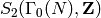It measures congruences between $f$ and elements of $S_2(\Gamma_0(N),\ZZ)$ orthogonal to $f$ .

EXAMPLES:

sage: E = EllipticCurve('37a')
sage: E.congruence_number()
2
sage: E.congruence_number()
2
sage: E = EllipticCurve('54b')
sage: E.congruence_number()
6
sage: E.modular_degree()
2
sage: E = EllipticCurve('242a1')
sage: E.modular_degree()
16
sage: E.congruence_number()  # long time
176

It is a theorem of Ribet that the congruence number is equal to the modular degree in the case of square free conductor. It is a conjecture of Agashe, Ribet, and Stein that $ord_p(c_f/m_f) \le ord_p(N)/2$ .

TESTS:

sage: E = EllipticCurve('11a')
sage: E.congruence_number()
1

cremona_label(space=False)¶

Return the Cremona label associated to (the minimal model) of this curve, if it is known. If not, raise a RuntimeError exception.

EXAMPLES:

sage: E=EllipticCurve('389a1')
sage: E.cremona_label()
'389a1'

The default database only contains conductors up to 10000, so any curve with conductor greater than that will cause an error to be raised. The optional package ‘database_cremona_ellcurve-20071019’ contains more curves, with conductors up to 130000.

sage: E = EllipticCurve([1, -1, 0, -79, 289])
sage: E.conductor()
234446
sage: E.cremona_label()
...
RuntimeError: Cremona label not known for Elliptic Curve defined by y^2 + x*y = x^3 - x^2 - 79*x + 289 over Rational Field.

database_curve()¶

Return the curve in the elliptic curve database isomorphic to this curve, if possible. Otherwise raise a RuntimeError exception.

EXAMPLES:

sage: E = EllipticCurve([0,1,2,3,4])
sage: E.database_curve()
Elliptic Curve defined by y^2  = x^3 + x^2 + 3*x + 5 over Rational Field

Note

The model of the curve in the database can be different from the Weierstrass model for this curve, e.g., database models are always minimal.

elliptic_exponential(z, embedding=None)¶

Computes the elliptic exponential of a complex number with respect to the elliptic curve.

INPUT:

z (complex) – a complex number
embedding - ignored (for compatibility with the period_lattice function for elliptic_curve_number_field)

OUTPUT:

The image of $z$ modulo $L$ under the Weierstrass parametrization $\CC/L \to E(\CC)$ .

Note

The precision is that of the input z, or the default precision of 53 bits if z is exact.

EXAMPLES:

sage: E = EllipticCurve([1,1,1,-8,6])
sage: P = E([0,2])
sage: z = P.elliptic_logarithm() # default precision is 100 here
sage: E.elliptic_exponential(z)
(-7.4445166...e-30 : 2.0000000000000000000000000000 : 1.0000000000000000000000000000)
sage: z = E([0,2]).elliptic_logarithm(precision=200)
sage: E.elliptic_exponential(z)
(-1.07731...e-60 : 2.0000000000000000000000000000000000000000000000000000000000 : 1.0000000000000000000000000000000000000000000000000000000000)

sage: E = EllipticCurve('389a')
sage: Q = E([3,5])
sage: E.elliptic_exponential(Q.elliptic_logarithm())
(3.0000000000000000000000000000 : 5.0000000000000000000000000000 : 1.0000000000000000000000000000)
sage: P = E([-1,1])
sage: P.elliptic_logarithm()
0.47934825019021931612953301006 + 0.98586885077582410221120384908*I
sage: E.elliptic_exponential(P.elliptic_logarithm())
(-1.0000000000000000000000000000 + 4.3761255...e-31*I : 1.0000000000000000000000000000 - 1.4587084969798853407242847702e-31*I : 1.0000000000000000000000000000)

Some torsion examples:

sage: w1,w2 = E.period_lattice().basis()
sage: E.two_division_polynomial().roots(CC,multiplicities=False)
[-2.0403022002854..., 0.13540924022175..., 0.90489296006371...]
sage: [E.elliptic_exponential((a*w1+b*w2)/2)[0] for a,b in [(0,1),(1,1),(1,0)]]
[-2.0403022002854..., 0.13540924022175..., 0.90489296006371...]

sage: E.division_polynomial(3).roots(CC,multiplicities=False)
[-2.88288879135...,
1.39292799513...,
0.078313731444316... - 0.492840991709...*I,
0.078313731444316... + 0.492840991709...*I]
sage: [E.elliptic_exponential((a*w1+b*w2)/3)[0] for a,b in [(0,1),(1,0),(1,1),(2,1)]]
[-2.8828887913533..., 1.39292799513138,
0.0783137314443... - 0.492840991709...*I,
0.0783137314443... + 0.492840991709...*I]

Observe that this is a group homomorphism (modulo rounding error):

sage: z = CC.random_element()
sage: 2 * E.elliptic_exponential(z)
(2.04119347066305 - 1.10251372205166*I : 2.23105000976838 - 2.69795281735238*I : 1.00000000000000)
sage: E.elliptic_exponential(2 * z)
(2.04119347066305 - 1.10251372205167*I : 2.23105000976839 - 2.69795281735236*I : 1.00000000000000)

eval_modular_form(points, prec)¶

Evaluate the modular form of this elliptic curve at points in CC

INPUT:

points - a list of points in the half-plane of convergence
prec - precision

OUTPUT: A list of values L(E,s) for s in points

Note

Better examples are welcome.

EXAMPLES:

sage: E=EllipticCurve('37a1')
sage: E.eval_modular_form([1.5+I,2.0+I,2.5+I],0.000001)
[0, 0, 0]

galois_representation()¶

The compatible family of the Galois representation attached to this elliptic curve.

Given an elliptic curve $E$ over $\QQ$ and a rational prime number $p$ , the $p^n$ -torsion $E[p^n]$ points of $E$ is a representation of the absolute Galois group of $\QQ$ . As $n$ varies we obtain the Tate module $T_p E$ which is a a representation of $G_K$ on a free $\ZZ_p$ -module of rank $2$ . As $p$ varies the representations are compatible.

EXAMPLES:

sage: rho = EllipticCurve('11a1').galois_representation()
sage: rho
Compatible family of Galois representations associated to the Elliptic Curve defined by y^2 + y = x^3 - x^2 - 10*x - 20 over Rational Field
sage: rho.is_irreducible(7)
True
sage: rho.is_irreducible(5)
False
sage: rho.is_surjective(11)
True
sage: rho.non_surjective()
[5]
sage: rho = EllipticCurve('37a1').galois_representation()
sage: rho.non_surjective()
[]
sage: rho = EllipticCurve('27a1').galois_representation()
sage: rho.is_irreducible(7)
True
sage: rho.non_surjective()   # cm-curve
[0]

gens(verbose=False, rank1_search=10, algorithm='mwrank_lib', only_use_mwrank=True, proof=None, use_database=True, descent_second_limit=12)¶

Compute and return generators for the Mordell-Weil group E(Q) modulo torsion.

Warning

If the program fails to give a provably correct result, it prints a warning message, but does not raise an exception. Use the gens_certain command to find out if this warning message was printed.

INPUT:

verbose - (default: None), if specified changes the verbosity of mwrank computations.
rank1_search - (default: 10), if the curve has analytic rank 1, try to find a generator by a direct search up to this logarithmic height. If this fails the usual mwrank procedure is called. algorithm -
- 'mwrank_shell' (default) - call mwrank shell command
- 'mwrank_lib' - call mwrank c library
only_use_mwrank - bool (default True) if False, attempts to first use more naive, natively implemented methods.
proof - bool or None (default None, see proof.elliptic_curve or sage.structure.proof).
use_database - bool (default True) if True, attempts to find curve and gens in the (optional) database
descent_second_limit - (default: 12)- used in 2-descent

OUTPUT:

generators - List of generators for the Mordell-Weil group modulo torsion.

IMPLEMENTATION: Uses Cremona’s mwrank C library.

EXAMPLES:

sage: E = EllipticCurve('389a')
sage: E.gens()                 # random output    
[(-1 : 1 : 1), (0 : 0 : 1)]

A non-integral example:

sage: E = EllipticCurve([-3/8,-2/3])
sage: E.gens() # random (up to sign)
[(10/9 : 29/54 : 1)]

A non-minimal example:

sage: E = EllipticCurve('389a1')
sage: E1 = E.change_weierstrass_model([1/20,0,0,0]); E1
Elliptic Curve defined by y^2 + 8000*y = x^3 + 400*x^2 - 320000*x over Rational Field
sage: E1.gens() # random (if database not used)
[(-400 : 8000 : 1), (0 : -8000 : 1)]

gens_certain()¶

Return True if the generators have been proven correct.

EXAMPLES:

sage: E=EllipticCurve('37a1')
sage: E.gens()                   # random (up to sign)
[(0 : -1 : 1)]
sage: E.gens_certain()
True

global_integral_model()¶

Return a model of self which is integral at all primes.

EXAMPLES:

sage: E = EllipticCurve([0, 0, 1/216, -7/1296, 1/7776])
sage: F = E.global_integral_model(); F
Elliptic Curve defined by y^2 + y = x^3 - 7*x + 6 over Rational Field
sage: F == EllipticCurve('5077a1')
True

has_cm()¶

Returns True iff this elliptic curve has Complex Multiplication.

EXAMPLES:

sage: E=EllipticCurve('37a1')
sage: E.has_cm()
False
sage: E=EllipticCurve('32a1')
sage: E.has_cm()
True
sage: E.j_invariant()
1728

has_good_reduction_outside_S(S=[])¶

Tests if this elliptic curve has good reduction outside $S$ .

INPUT:

S - list of primes (default: empty list).

Note

Primality of elements of S is not checked, and the output is undefined if S is not a list or contains non-primes.

This only tests the given model, so should only be applied to minimal models.

EXAMPLES:

sage: EllipticCurve('11a1').has_good_reduction_outside_S([11])
True
sage: EllipticCurve('11a1').has_good_reduction_outside_S([2])
False
sage: EllipticCurve('2310a1').has_good_reduction_outside_S([2,3,5,7])
False
sage: EllipticCurve('2310a1').has_good_reduction_outside_S([2,3,5,7,11])
True

heegner_discriminants(bound)¶

Return the list of self’s Heegner discriminants between -1 and -bound.

INPUT:

bound (int) - upper bound for -discriminant

OUTPUT: The list of Heegner discriminants between -1 and -bound for the given elliptic curve.

EXAMPLES:

sage: E=EllipticCurve('11a')
sage: E.heegner_discriminants(30)                     # indirect doctest
[-7, -8, -19, -24]

heegner_discriminants_list(n)¶

Return the list of self’s first $n$ Heegner discriminants smaller than -5.

INPUT:

n (int) - the number of discriminants to compute

OUTPUT: The list of the first n Heegner discriminants smaller than -5 for the given elliptic curve.

EXAMPLE:

sage: E=EllipticCurve('11a')
sage: E.heegner_discriminants_list(4)                     # indirect doctest
[-7, -8, -19, -24]

heegner_index(D, min_p=2, prec=5, descent_second_limit=12, verbose_mwrank=False)¶

Return an interval that contains the index of the Heegner point $y_K$ in the group of $K$ -rational points modulo torsion on this elliptic curve, computed using the Gross-Zagier formula and/or a point search, or possibly half the index if the rank is greater than one.

Note

If min_p is bigger than 2 then the index can be off by any prime less than min_p. This function returns the index divided by $2$ exactly when the rank of $E(K)$ is greater than 1 and $E(\QQ)_{/tor} \oplus E^D(\QQ)_{/tor}$ has index $2$ in $E(K)_{/tor}$ , where the second factor undergoes a twist.

INPUT:

D (int) - Heegner discriminant
min_p (int) - (default: 2) only rule out primes = min_p dividing the index.
verbose_mwrank (bool) - (default: False); print lots of mwrank search status information when computing regulator
prec (int) - (default: 5), use prec*sqrt(N) + 20 terms of L-series in computations, where N is the conductor.
descent_second_limit - (default: 12)- used in 2-descent when computing regulator of the twist

OUTPUT: an interval that contains the index, or half the index

EXAMPLES:

sage: E = EllipticCurve('11a')
sage: E.heegner_discriminants(50)
[-7, -8, -19, -24, -35, -39, -40, -43]
sage: E.heegner_index(-7)
1.00000?

sage: E = EllipticCurve('37b')
sage: E.heegner_discriminants(100)
[-3, -4, -7, -11, -40, -47, -67, -71, -83, -84, -95]
sage: E.heegner_index(-95)          # long time (1 second)
2.00000?

This tests doing direct computation of the Mordell-Weil group.

sage: EllipticCurve('675b').heegner_index(-11)
3.0000?

Currently discriminants -3 and -4 are not supported:

sage: E.heegner_index(-3)
...
ArithmeticError: Discriminant (=-3) must not be -3 or -4.

The curve 681b returns the true index, which is $3$ :

sage: E = EllipticCurve('681b')
sage: I = E.heegner_index(-8); I
3.0000?

In fact, whenever the returned index has a denominator of $2$ , the true index is got by multiplying the returned index by $2$ . Unfortunately, this is not an if and only if condition, i.e., sometimes the index must be multiplied by $2$ even though the denominator is not $2$ .

This example demonstrates the $descent_second_limit$ option, which can be used to fine tune the 2-descent used to compute the regulator of the twist:

sage: E = EllipticCurve([0, 0, 1, -34874, -2506691])
sage: E.heegner_index(-8)
...
RuntimeError: ...

However when we search higher, we find the points we need:

sage: E.heegner_index(-8, descent_second_limit=16)
1.00000?

heegner_index_bound(D=0, prec=5, max_height=None)¶

Assume self has rank 0.

Return a list $v$ of primes such that if an odd prime $p$ divides the index of the Heegner point in the group of rational points modulo torsion, then $p$ is in $v$ .

If 0 is in the interval of the height of the Heegner point computed to the given prec, then this function returns $v = 0$ . This does not mean that the Heegner point is torsion, just that it is very likely torsion.

If we obtain no information from a search up to max_height, e.g., if the Siksek et al. bound is bigger than max_height, then we return $v = -1$ .

INPUT:

D (int) - (default: 0) Heegner discriminant; if 0, use the first discriminant -4 that satisfies the Heegner hypothesis
verbose (bool) - (default: True)
prec (int) - (default: 5), use $prec \cdot \sqrt(N) + 20$ terms of $L$ -series in computations, where $N$ is the conductor.
max_height (float) - should be = 21; bound on logarithmic naive height used in point searches. Make smaller to make this function faster, at the expense of possibly obtaining a worse answer. A good range is between 13 and 21.

OUTPUT:

v - list or int (bad primes or 0 or -1)
D - the discriminant that was used (this is useful if $D$ was automatically selected).

EXAMPLES:

sage: E = EllipticCurve('11a1')
sage: E.heegner_index_bound()
([2], -7)

heegner_point(D, c=1, f=None, check=True)¶

Returns the Heegner point on this curve associated to the quadratic imaginary field $K=\QQ(\sqrt{D})$ .

If the optional parameter $c$ is given, returns the higher Heegner point associated to the order of conductor $c$ .

INPUT:

- `D`        -- a Heegner discriminant

- `c`        -- (default: 1) conductor, must be coprime to `DN`

- `f`        -- binary quadratic form or 3-tuple `(A,B,C)` of coefficients
                of `AX^2 + BXY + CY^2`

- ``check``  -- bool (default: True)

OUTPUT:

The Heegner point `y_c`.

EXAMPLES:

sage: E = EllipticCurve('37a')
sage: E.heegner_discriminants_list(10)
[-7, -11, -40, -47, -67, -71, -83, -84, -95, -104]
sage: P = E.heegner_point(-7); P                          # indirect doctest
Heegner point of discriminant -7 on elliptic curve of conductor 37
sage: P.point_exact()
(0 : 0 : 1)
sage: P.curve()
Elliptic Curve defined by y^2 + y = x^3 - x over Rational Field
sage: P = E.heegner_point(-40).point_exact(); P
(a : a - 2 : 1)
sage: P = E.heegner_point(-47).point_exact(); P
(a : a^4 + a - 1 : 1)
sage: P[0].parent()
Number Field in a with defining polynomial x^5 - x^4 + x^3 + x^2 - 2*x + 1

Working out the details manually:

sage: P = E.heegner_point(-47).numerical_approx(prec=200)
sage: f = algdep(P[0], 5); f
x^5 - x^4 + x^3 + x^2 - 2*x + 1
sage: f.discriminant().factor()
47^2

The Heegner hypothesis is checked:

sage: E = EllipticCurve('389a'); P = E.heegner_point(-5,7);
...
ValueError: N (=389) and D (=-5) must satisfy the Heegner hypothesis

We can specify the quadratic form:

sage: P = EllipticCurve('389a').heegner_point(-7, 5, (778,925,275)); P
Heegner point of discriminant -7 and conductor 5 on elliptic curve of conductor 389
sage: P.quadratic_form()
778*x^2 + 925*x*y + 275*y^2

heegner_point_height(D, prec=2)¶

Use the Gross-Zagier formula to compute the Neron-Tate canonical height over $K$ of the Heegner point corresponding to $D$ , as an interval (it’s computed to some precision using $L$ -functions).

INPUT:

D (int) - fundamental discriminant (=/= -3, -4)
prec (int) - (default: 2), use $prec \cdot \sqrt(N) + 20$ terms of $L$ -series in computations, where $N$ is the conductor.

OUTPUT: Interval that contains the height of the Heegner point.

EXAMPLE:

sage: E = EllipticCurve('11a')
sage: E.heegner_point_height(-7)
0.22227?

heegner_sha_an(D, prec=53)¶

Return the conjectural (analytic) order of Sha for E over the field $K=\QQ(\sqrt{D})$ .

INPUT:

$D$ – negative integer; the Heegner discriminant
prec – integer (default: 53); bits of precision to compute analytic order of Sha

OUTPUT:

(floating point number) an approximation to the conjectural order of Sha.

Note

Often you’ll want to do proof.elliptic_curve(False) when using this function, since often the twisted elliptic curves that come up have enormous conductor, and Sha is nontrivial, which makes provably finding the Mordell-Weil group using 2-descent difficult.

EXAMPLES:

An example where E has conductor 11:

sage: E = EllipticCurve('11a')
sage: E.heegner_sha_an(-7)                                  # long
1.00000000000000

The cache works:

sage: E.heegner_sha_an(-7) is E.heegner_sha_an(-7)          # long
True

Lower precision:

sage: E.heegner_sha_an(-7,10)                               # long
1.0

Checking that the cache works for any precision:

sage: E.heegner_sha_an(-7,10) is E.heegner_sha_an(-7,10)    # long
True

Next we consider a rank 1 curve with nontrivial Sha over the quadratic imaginary field $K$ ; however, there is no Sha for $E$ over $\QQ$ or for the quadratic twist of $E$ :

sage: E = EllipticCurve('37a')
sage: E.heegner_sha_an(-40)                                 # long
4.00000000000000
sage: E.quadratic_twist(-40).sha().an()                     # long
1
sage: E.sha().an()                                          # long
1

A rank 2 curve:

sage: E = EllipticCurve('389a')                             # long
sage: E.heegner_sha_an(-7)                                  # long
1.00000000000000

If we remove the hypothesis that $E(K)$ has rank 1 in Conjecture 2.3 in [Gross-Zagier, 1986, page 311], then that conjecture is false, as the following example shows:

sage: E = EllipticCurve('65a')                              # long
sage: E.heegner_sha_an(-56)                                 # long
1.00000000000000
sage: E.torsion_order()                                     # long
2
sage: E.tamagawa_product()                                  # long
1
sage: E.quadratic_twist(-56).rank()                         # long
2

height(precision=None)¶

Returns the real height of this elliptic curve. This is used in integral_points()

INPUT:

precision - desired real precision of the result (default real precision if None)

EXAMPLES:

sage: E=EllipticCurve('5077a1')
sage: E.height()               
17.4513334798896
sage: E.height(100)
17.451333479889612702508579399
sage: E=EllipticCurve([0,0,0,0,1])
sage: E.height()                  
1.38629436111989
sage: E=EllipticCurve([0,0,0,1,0])
sage: E.height()                  
7.45471994936400

height_pairing_matrix(points=None, precision=None)¶

Returns the height pairing matrix of the given points on this curve, which must be defined over $\QQ$ .

INPUT:

points - either a list of points, which must be on this curve, or (default) None, in which case self.gens() will be used. precision - number of bits of precision of result (default: None, for default RealField precision)

EXAMPLES:

sage: E = EllipticCurve([0, 0, 1, -1, 0])
sage: E.height_pairing_matrix()
[0.0511114082399688]

For rank 0 curves, the result is a valid 0x0 matrix:

sage: EllipticCurve('11a').height_pairing_matrix()
[]
sage: E=EllipticCurve('5077a1')
sage: E.height_pairing_matrix([E.lift_x(x) for x in [-2,-7/4,1]], precision=100)
[  1.3685725053539301120518194471  -1.3095767070865761992624519454 -0.63486715783715592064475542573]
[ -1.3095767070865761992624519454   2.7173593928122930896610589220   1.0998184305667292139777571432]
[-0.63486715783715592064475542573   1.0998184305667292139777571432  0.66820516565192793503314205089]

integral_model()¶

Return a model of self which is integral at all primes.

EXAMPLES:

sage: E = EllipticCurve([0, 0, 1/216, -7/1296, 1/7776])
sage: F = E.global_integral_model(); F
Elliptic Curve defined by y^2 + y = x^3 - 7*x + 6 over Rational Field
sage: F == EllipticCurve('5077a1')
True

integral_points(mw_base='auto', both_signs=False, verbose=False)¶

Computes all integral points (up to sign) on this elliptic curve.

INPUT:

mw_base - list of EllipticCurvePoint generating the Mordell-Weil group of E (default: ‘auto’ - calls self.gens())
both_signs - True/False (default False): if True the output contains both P and -P, otherwise only one of each pair.
verbose - True/False (default False): if True, some details of the computation are output

OUTPUT: A sorted list of all the integral points on E (up to sign unless both_signs is True)

Note

The complexity increases exponentially in the rank of curve E. The computation time (but not the output!) depends on the Mordell-Weil basis. If mw_base is given but is not a basis for the Mordell-Weil group (modulo torsion), integral points which are not in the subgroup generated by the given points will almost certainly not be listed.

EXAMPLES: A curve of rank 3 with no torsion points

sage: E=EllipticCurve([0,0,1,-7,6])
sage: P1=E.point((2,0)); P2=E.point((-1,3)); P3=E.point((4,6))
sage: a=E.integral_points([P1,P2,P3]); a  
[(-3 : 0 : 1), (-2 : 3 : 1), (-1 : 3 : 1), (0 : 2 : 1), (1 : 0 : 1), (2 : 0 : 1), (3 : 3 : 1), (4 : 6 : 1), (8 : 21 : 1), (11 : 35 : 1), (14 : 51 : 1), (21 : 95 : 1), (37 : 224 : 1), (52 : 374 : 1), (93 : 896 : 1), (342 : 6324 : 1), (406 : 8180 : 1), (816 : 23309 : 1)]

sage: a = E.integral_points([P1,P2,P3], verbose=True) 
Using mw_basis  [(2 : 0 : 1), (3 : -4 : 1), (8 : -22 : 1)]
e1,e2,e3:  -3.0124303725933... 1.0658205476962... 1.94660982489710
Minimal eigenvalue of height pairing matrix:  0.63792081458500...
x-coords of points on compact component with  -3 <=x<= 1
[-3, -2, -1, 0, 1]
x-coords of points on non-compact component with  2 <=x<= 6
[2, 3, 4]
starting search of remaining points using coefficient bound  5
x-coords of extra integral points:
[2, 3, 4, 8, 11, 14, 21, 37, 52, 93, 342, 406, 816]
Total number of integral points: 18

It is not necessary to specify mw_base; if it is not provided, then the Mordell-Weil basis must be computed, which may take much longer.

sage: E=EllipticCurve([0,0,1,-7,6])
sage: a=E.integral_points(both_signs=True); a
[(-3 : -1 : 1), (-3 : 0 : 1), (-2 : -4 : 1), (-2 : 3 : 1), (-1 : -4 : 1), (-1 : 3 : 1), (0 : -3 : 1), (0 : 2 : 1), (1 : -1 : 1), (1 : 0 : 1), (2 : -1 : 1), (2 : 0 : 1), (3 : -4 : 1), (3 : 3 : 1), (4 : -7 : 1), (4 : 6 : 1), (8 : -22 : 1), (8 : 21 : 1), (11 : -36 : 1), (11 : 35 : 1), (14 : -52 : 1), (14 : 51 : 1), (21 : -96 : 1), (21 : 95 : 1), (37 : -225 : 1), (37 : 224 : 1), (52 : -375 : 1), (52 : 374 : 1), (93 : -897 : 1), (93 : 896 : 1), (342 : -6325 : 1), (342 : 6324 : 1), (406 : -8181 : 1), (406 : 8180 : 1), (816 : -23310 : 1), (816 : 23309 : 1)]

An example with negative discriminant:

sage: EllipticCurve('900d1').integral_points() 
[(-11 : 27 : 1), (-4 : 34 : 1), (4 : 18 : 1), (16 : 54 : 1)]

Another example with rank 5 and no torsion points

sage: E=EllipticCurve([-879984,319138704])
sage: P1=E.point((540,1188)); P2=E.point((576,1836))
sage: P3=E.point((468,3132)); P4=E.point((612,3132))
sage: P5=E.point((432,4428))
sage: a=E.integral_points([P1,P2,P3,P4,P5]); len(a)  # long time (400s!)
54

The bug reported on trac #4525 is now fixed:

sage: EllipticCurve('91b1').integral_points()
[(-1 : 3 : 1), (1 : 0 : 1), (3 : 4 : 1)]

sage: [len(e.integral_points(both_signs=False)) for e in cremona_curves([11..100])] # long time
[2, 0, 2, 3, 2, 1, 3, 0, 2, 4, 2, 4, 3, 0, 0, 1, 2, 1, 2, 0, 2, 1, 0, 1, 3, 3, 1, 1, 4, 2, 3, 2, 0, 0, 5, 3, 2, 2, 1, 1, 1, 0, 1, 3, 0, 1, 0, 1, 1, 3, 6, 1, 2, 2, 2, 0, 0, 2, 3, 1, 2, 2, 1, 1, 0, 3, 2, 1, 0, 1, 0, 1, 3, 3, 1, 1, 5, 1, 0, 1, 1, 0, 1, 2, 0, 2, 0, 1, 1, 3, 1, 2, 2, 4, 4, 2, 1, 0, 0, 5, 1, 0, 1, 2, 0, 2, 2, 0, 0, 0, 1, 0, 3, 1, 5, 1, 2, 4, 1, 0, 1, 0, 1, 0, 1, 0, 2, 2, 0, 0, 1, 0, 1, 1, 4, 1, 0, 1, 1, 0, 4, 2, 0, 1, 1, 2, 3, 1, 1, 1, 1, 6, 2, 1, 1, 0, 2, 0, 6, 2, 0, 4, 2, 2, 0, 0, 1, 2, 0, 2, 1, 0, 3, 1, 2, 1, 4, 6, 3, 2, 1, 0, 2, 2, 0, 0, 5, 4, 1, 0, 0, 1, 0, 2, 2, 0, 0, 2, 3, 1, 3, 1, 1, 0, 1, 0, 0, 1, 2, 2, 0, 2, 0, 0, 1, 2, 0, 0, 4, 1, 0, 1, 1, 0, 1, 2, 0, 1, 4, 3, 1, 2, 2, 1, 1, 1, 1, 6, 3, 3, 3, 3, 1, 1, 1, 1, 1, 0, 7, 3, 0, 1, 3, 2, 1, 0, 3, 2, 1, 0, 2, 2, 6, 0, 0, 6, 2, 2, 3, 3, 5, 5, 1, 0, 6, 1, 0, 3, 1, 1, 2, 3, 1, 2, 1, 1, 0, 1, 0, 1, 0, 5, 5, 2, 2, 0, 0, 1, 0, 0, 0, 0, 1, 1, 1, 1]

The bug reported at #4897 is now fixed:

sage: [P[0] for P in EllipticCurve([0,0,0,-468,2592]).integral_points()]
[-24, -18, -14, -6, -3, 4, 6, 18, 21, 24, 36, 46, 102, 168, 186, 381, 1476, 2034, 67246]

Note

This function uses the algorithm given in [Co1].

REFERENCES:

[Co1] Cohen H., Number Theory Vol I: Tools and Diophantine Equations GTM 239, Springer 2007

AUTHORS:

Michael Mardaus (2008-07)
Tobias Nagel (2008-07)
John Cremona (2008-07)

integral_short_weierstrass_model()¶

Return a model of the form $y^2 = x^3 + ax + b$ for this curve with $a,b\in\ZZ$ .

EXAMPLES:

sage: E = EllipticCurve('17a1')
sage: E.integral_short_weierstrass_model()
Elliptic Curve defined by y^2  = x^3 - 11*x - 890 over Rational Field

integral_weierstrass_model()¶

Return a model of the form $y^2 = x^3 + ax + b$ for this curve with $a,b\in\ZZ$ .

Note that this function is deprecated, and that you should use integral_short_weierstrass_model instead as this will be disappearing in the near future.

EXAMPLES:

sage: E = EllipticCurve('17a1')
sage: E.integral_weierstrass_model() #random
doctest:1: DeprecationWarning: integral_weierstrass_model is deprecated, use integral_short_weierstrass_model instead!
Elliptic Curve defined by y^2  = x^3 - 11*x - 890 over Rational Field

integral_x_coords_in_interval(xmin, xmax)¶

Returns the set of integers $x$ with $xmin\le x\le xmax$ which are $x$ -coordinates of rational points on this curve.

INPUT:

xmin, xmax (integers) – two integers.

OUTPUT:

(set) The set of integers $x$ with $xmin\le x\le xmax$ which are $x$ -coordinates of rational points on the elliptic curve.

EXAMPLES:

sage: E = EllipticCurve([0, 0, 1, -7, 6])
sage: xset = E.integral_x_coords_in_interval(-100,100)
sage: xlist = list(xset); xlist.sort(); xlist
[-3, -2, -1, 0, 1, 2, 3, 4, 8, 11, 14, 21, 37, 52, 93]

TODO: re-implement this using the much faster point searching implemented in Stoll’s ratpoints program.

is_global_integral_model()¶

Return true iff self is integral at all primes.

EXAMPLES:

sage: E=EllipticCurve([1/2,1/5,1/5,1/5,1/5])
sage: E.is_global_integral_model()
False
sage: Emin=E.global_integral_model()
sage: Emin.is_global_integral_model()
True

is_good(p, check=True)¶

Return True if $p$ is a prime of good reduction for $E$ .

INPUT:

p - a prime

OUTPUT: bool

EXAMPLES:

sage: e = EllipticCurve('11a')
sage: e.is_good(-8)
...
ValueError: p must be prime
sage: e.is_good(-8, check=False)
True

is_integral()¶

Returns True if this elliptic curve has integral coefficients (in Z)

EXAMPLES:

sage: E=EllipticCurve(QQ,[1,1]); E
Elliptic Curve defined by y^2 = x^3 + x + 1 over Rational Field
sage: E.is_integral()
True
sage: E2=E.change_weierstrass_model(2,0,0,0); E2
Elliptic Curve defined by y^2 = x^3 + 1/16*x + 1/64 over Rational Field
sage: E2.is_integral()
False

is_irreducible(p)¶

Return True if the mod p representation is irreducible.

Note that this function is deprecated, and that you should use galois_representation().is_irreducible(p) instead as this will be disappearing in the near future.

EXAMPLES:

sage: EllipticCurve('20a1').is_irreducible(7) #random
doctest:1: DeprecationWarning: is_irreducible is deprecated, use galois_representation().is_irreducible(p) instead!
True

is_isogenous(other, proof=True, maxp=200)¶

Returns whether or not self is isogenous to other.

INPUT:

other – another elliptic curve.
proof (default True) – If False, the function will return True whenever the two curves have the same conductor and are isogenous modulo $p$ for $p$ up to maxp. If True, this test is followed by a rigorous test (which may be more time-consuming).
maxp (int, default 200) – The maximum prime $p$ for which isogeny modulo $p$ will be checked.

OUTPUT:

(bool) True if there is an isogeny from curve self to curve other.

METHOD:

First the conductors are compared as well as the Traces of Frobenius for good primes up to maxp. If any of these tests fail, False is returned. If they all pass and proof is False then True is returned, otherwise a complete set of curves isogenous to self is computed and other is checked for isomorphism with any of these,

EXAMPLES:

sage: E1 = EllipticCurve('14a1')   
sage: E6 = EllipticCurve('14a6')                
sage: E1.is_isogenous(E6)
True
sage: E1.is_isogenous(EllipticCurve('11a1'))     
False

sage: EllipticCurve('37a1').is_isogenous(EllipticCurve('37b1'))
False

sage: E = EllipticCurve([2, 16])          
sage: EE = EllipticCurve([87, 45])       
sage: E.is_isogenous(EE)
False

is_local_integral_model(*p)¶

Tests if self is integral at the prime $p$ , or at all the primes if $p$ is a list or tuple of primes

EXAMPLES:

sage: E=EllipticCurve([1/2,1/5,1/5,1/5,1/5])
sage: [E.is_local_integral_model(p) for p in (2,3,5)]
[False, True, False]
sage: E.is_local_integral_model(2,3,5)
False
sage: Eint2=E.local_integral_model(2)
sage: Eint2.is_local_integral_model(2)
True

is_minimal()¶

Return True iff this elliptic curve is a reduced minimal model.

The unique minimal Weierstrass equation for this elliptic curve. This is the model with minimal discriminant and $a_1,a_2,a_3 \in \{0,\pm 1\}$ .

TO DO: This is not very efficient since it just computes the minimal model and compares. A better implementation using the Kraus conditions would be preferable.

EXAMPLES:

sage: E=EllipticCurve([10,100,1000,10000,1000000])
sage: E.is_minimal()
False
sage: E=E.minimal_model()
sage: E.is_minimal()
True

is_ordinary(p, ell=None)¶

Return True precisely when the mod-p representation attached to this elliptic curve is ordinary at ell.

INPUT:

p - a prime ell - a prime (default: p)

OUTPUT: bool

EXAMPLES:

sage: E=EllipticCurve('37a1')
sage: E.is_ordinary(37)
True
sage: E=EllipticCurve('32a1')
sage: E.is_ordinary(2)
False
sage: [p for p in prime_range(50) if E.is_ordinary(p)]
[5, 13, 17, 29, 37, 41]

is_p_integral(p)¶

Returns True if this elliptic curve has $p$ -integral coefficients.

INPUT:

p - a prime integer

EXAMPLES:

sage: E=EllipticCurve(QQ,[1,1]); E
Elliptic Curve defined by y^2 = x^3 + x + 1 over Rational Field
sage: E.is_p_integral(2)
True
sage: E2=E.change_weierstrass_model(2,0,0,0); E2
Elliptic Curve defined by y^2 = x^3 + 1/16*x + 1/64 over Rational Field
sage: E2.is_p_integral(2)
False
sage: E2.is_p_integral(3)
True

is_p_minimal(p)¶

Tests if curve is p-minimal at a given prime p.

INPUT: p - a primeOUTPUT: True - if curve is p-minimal

False - if curve isn’t p-minimal

EXAMPLES:

sage: E = EllipticCurve('441a2')
sage: E.is_p_minimal(7)
True

sage: E = EllipticCurve([0,0,0,0,(2*5*11)**10])
sage: [E.is_p_minimal(p) for p in prime_range(2,24)]
[False, True, False, True, False, True, True, True, True]

is_reducible(p)¶

Return True if the mod-p representation attached to E is reducible.

Note that this function is deprecated, and that you should use galois_representation().is_reducible(p) instead as this will be disappearing in the near future.

EXAMPLES:

sage: EllipticCurve('20a1').is_reducible(3) #random
doctest:1: DeprecationWarning: is_reducible is deprecated, use galois_representation().is_reducible(p) instead!
True

is_semistable()¶

Return True iff this elliptic curve is semi-stable at all primes.

EXAMPLES:

sage: E=EllipticCurve('37a1')
sage: E.is_semistable()
True
sage: E=EllipticCurve('90a1')
sage: E.is_semistable()
False

is_supersingular(p, ell=None)¶

Return True precisely when p is a prime of good reduction and the mod-p representation attached to this elliptic curve is supersingular at ell.

INPUT:

p - a prime ell - a prime (default: p)

OUTPUT: bool

EXAMPLES:

sage: E=EllipticCurve('37a1')
sage: E.is_supersingular(37)
False
sage: E=EllipticCurve('32a1')
sage: E.is_supersingular(2)
False
sage: E.is_supersingular(7)
True
sage: [p for p in prime_range(50) if E.is_supersingular(p)]
[3, 7, 11, 19, 23, 31, 43, 47]

is_surjective(p, A=1000)¶

Returns true if the mod p representation is surjective

Note that this function is deprecated, and that you should use galois_representation().is_surjective(p) instead as this will be disappearing in the near future.

EXAMPLES:

sage: EllipticCurve('20a1').is_surjective(7) #random
doctest:1: DeprecationWarning: is_surjective is deprecated, use galois_representation().is_surjective(p) instead!
True

isogenies_prime_degree(l=None)¶

Returns a list of $\ell$ -isogenies from self, where $\ell$ is a prime.

INPUT:

l – either None or a prime or a list of primes.

OUTPUT:

(list) $\ell$ -isogenies for the given $\ell$ or if $\ell$ is None, all $\ell$ -isogenies.

Note

The codomains of the isogenies returned are standard minimal models. This is because the functions isogenies_prime_degree_genus_0() and isogenies_sporadic_Q() are implemented that way for curves defined over $\QQ$ .

EXAMPLES:

sage: E = EllipticCurve([45,32])                        
sage: E.isogenies_prime_degree()
[]
sage: E = EllipticCurve(j = -262537412640768000) 
sage: E.isogenies_prime_degree()
[Isogeny of degree 163 from Elliptic Curve defined by y^2 + y = x^3 - 2174420*x + 1234136692 over Rational Field to Elliptic Curve defined by y^2 + y = x^3 - 57772164980*x - 5344733777551611 over Rational Field]
sage: E1 = E.quadratic_twist(6584935282)
sage: E1.isogenies_prime_degree()
[Isogeny of degree 163 from Elliptic Curve defined by y^2 = x^3 - 94285835957031797981376080*x + 352385311612420041387338054224547830898 over Rational Field to Elliptic Curve defined by y^2 = x^3 - 2505080375542377840567181069520*x - 1526091631109553256978090116318797845018020806 over Rational Field]

sage: E = EllipticCurve('14a1')                                   
sage: E.isogenies_prime_degree(2)
[Isogeny of degree 2 from Elliptic Curve defined by y^2 + x*y + y = x^3 + 4*x - 6 over Rational Field to Elliptic Curve defined by y^2 + x*y + y = x^3 - 36*x - 70 over Rational Field]
sage: E.isogenies_prime_degree(3)            
[Isogeny of degree 3 from Elliptic Curve defined by y^2 + x*y + y = x^3 + 4*x - 6 over Rational Field to Elliptic Curve defined by y^2 + x*y + y = x^3 - x over Rational Field, Isogeny of degree 3 from Elliptic Curve defined by y^2 + x*y + y = x^3 + 4*x - 6 over Rational Field to Elliptic Curve defined by y^2 + x*y + y = x^3 - 171*x - 874 over Rational Field]
sage: E.isogenies_prime_degree(5)
[]
sage: E.isogenies_prime_degree(11)
[]
sage: E.isogenies_prime_degree(29)
[]
sage: E.isogenies_prime_degree(4) 
...
ValueError: 4 is not prime.

isogeny_class(algorithm='sage', verbose=False, fill_matrix=True)¶

Returns all curves over $\QQ$ isogenous to this elliptic curve.

INPUT:

verbose – bool (default: False): ignored unless algorithm == “mwrank”, in which case it is passed to the isogeny class function in mwrank.
algorithm - string: one of the following:
- “mwrank” - (default) use the mwrank C++ library
- “database” - use the Cremona database (only works if curve is isomorphic to a curve in the database)
- “sage” - use the native Sage implementation.
fill_matrix – bool (default: True): See below.

OUTPUT:

Tuple (list of curves, matrix of integers). The sorted list of all curves isogenous to self is returned. If algorithm is not “database”, the isogeny matrix is also returned, otherwise None is returned as the second return value. When fill_matrix is True (default) the $(i,j)$ entry of the matrix is a positive integer giving the least degree of a cyclic isogeny from curve $i$ to curve $j$ (in particular, the diagonal entries are all $1$ ). When fill_matrix is False, the non-prime entries are replaced by $0$ (used in the isogeny_graph() function).

Note

The ordering depends on which algorithm is used.

Note

The curves returned are all standard minimal models.

Warning

With algorithm “mwrank”, the result is not provably correct, in the sense that when the numbers are huge isogenies could be missed because of precision issues. Using algorithm “sage” avoids this problem, though is slower.

EXAMPLES:

sage: I, A = EllipticCurve('37b').isogeny_class('mwrank')  
sage: I   # randomly ordered 
[Elliptic Curve defined by y^2 + y = x^3 + x^2 - 23*x - 50 over Rational Field,
 Elliptic Curve defined by y^2 + y = x^3 + x^2 - 1873*x - 31833 over Rational Field,
 Elliptic Curve defined by y^2 + y = x^3 + x^2 - 3*x +1 over Rational Field]
sage: A
[1 3 3]
[3 1 9]
[3 9 1]

sage: I, _ = EllipticCurve('37b').isogeny_class('database'); I
[Elliptic Curve defined by y^2 + y = x^3 + x^2 - 1873*x - 31833 over Rational Field,
 Elliptic Curve defined by y^2 + y = x^3 + x^2 - 23*x - 50 over Rational Field,
 Elliptic Curve defined by y^2 + y = x^3 + x^2 - 3*x + 1 over Rational Field]

This is an example of a curve with a $37$ -isogeny:

sage: E = EllipticCurve([1,1,1,-8,6])
sage: E.isogeny_class ()
([Elliptic Curve defined by y^2 + x*y + y = x^3 + x^2 - 8*x + 6 over Rational Field, Elliptic Curve defined by y^2 + x*y + y = x^3 + x^2 - 208083*x - 36621194 over Rational Field], [ 1 37]
[37  1])

This curve had numerous $2$ -isogenies:

sage: e=EllipticCurve([1,0,0,-39,90])
sage: e.isogeny_class ()
([Elliptic Curve defined by y^2 + x*y = x^3 - 39*x + 90 over Rational Field, Elliptic Curve defined by y^2 + x*y = x^3 - 4*x - 1 over Rational Field, Elliptic Curve defined by y^2 + x*y = x^3 + x over Rational Field, Elliptic Curve defined by y^2 + x*y = x^3 - 49*x - 136 over Rational Field, Elliptic Curve defined by y^2 + x*y = x^3 - 34*x - 217 over Rational Field, Elliptic Curve defined by y^2 + x*y = x^3 - 784*x - 8515 over Rational Field], [1 2 4 4 8 8]
[2 1 2 2 4 4]
[4 2 1 4 8 8]
[4 2 4 1 2 2]
[8 4 8 2 1 4]
[8 4 8 2 4 1])

See http://math.harvard.edu/~elkies/nature.html for more interesting examples of isogeny structures.

sage: E = EllipticCurve(j = -262537412640768000)
sage: E.isogeny_class(algorithm="sage")
([Elliptic Curve defined by y^2 + y = x^3 - 2174420*x + 1234136692 over Rational Field, Elliptic Curve defined by y^2 + y = x^3 - 57772164980*x - 5344733777551611 over Rational Field], [  1 163]
[163   1])

For large examples, the “mwrank” algorithm may fail to find some isogenies since it works in fixed precision:

sage: E1 = E.quadratic_twist(6584935282)
sage: E1.isogeny_class(algorithm="mwrank")
([Elliptic Curve defined by y^2 = x^3 - 94285835957031797981376080*x + 352385311612420041387338054224547830898 over Rational Field],
[1])

Since the result is cached, this looks no different:

sage: E1.isogeny_class(algorithm="sage")
([Elliptic Curve defined by y^2 = x^3 - 94285835957031797981376080*x + 352385311612420041387338054224547830898 over Rational Field],
[1])

But resetting the curve shows that the native algorithm is better:

 sage: E1 = E.quadratic_twist(6584935282)
 sage: E1.isogeny_class(algorithm="sage")
 ([Elliptic Curve defined by y^2 = x^3 - 94285835957031797981376080*x + 352385311612420041387338054224547830898 over Rational Field,
 Elliptic Curve defined by y^2 = x^3 - 2505080375542377840567181069520*x - 1526091631109553256978090116318797845018020806 over Rational Field],
 [  1 163]
 [163   1])
sage: E1.conductor()
18433092966712063653330496

sage: E = EllipticCurve('14a1')                 
sage: E.isogeny_class(algorithm="sage")            
([Elliptic Curve defined by y^2 + x*y + y = x^3 + 4*x - 6 over Rational Field, Elliptic Curve defined by y^2 + x*y + y = x^3 - 36*x - 70 over Rational Field, Elliptic Curve defined by y^2 + x*y + y = x^3 - x over Rational Field, Elliptic Curve defined by y^2 + x*y + y = x^3 - 171*x - 874 over Rational Field, Elliptic Curve defined by y^2 + x*y + y = x^3 - 11*x + 12 over Rational Field, Elliptic Curve defined by y^2 + x*y + y = x^3 - 2731*x - 55146 over Rational Field], [ 1  2  3  3  6  6]
[ 2  1  6  6  3  3]
[ 3  6  1  9  2 18]
[ 3  6  9  1 18  2]
[ 6  3  2 18  1  9]
[ 6  3 18  2  9  1])

isogeny_degree(other)¶

Returns the minimal degree of an isogeny between self and other.

INPUT:

other – another elliptic curve.

OUTPUT:

(int) The minimal degree of an isogeny from self to other, or 0 if the curves are not isogenous.

EXAMPLES:

sage: E = EllipticCurve([-1056, 13552])   
sage: E2 = EllipticCurve([-127776, -18037712])
sage: E.isogeny_degree(E2)
11

sage: E1 = EllipticCurve('14a1')   
sage: E2 = EllipticCurve('14a2')                 
sage: E3 = EllipticCurve('14a3')                 
sage: E4 = EllipticCurve('14a4')                 
sage: E5 = EllipticCurve('14a5')                 
sage: E6 = EllipticCurve('14a6')
sage: E3.isogeny_degree(E1)
3
sage: E3.isogeny_degree(E2)
6
sage: E3.isogeny_degree(E3)
1
sage: E3.isogeny_degree(E4)
9
sage: E3.isogeny_degree(E5)
2
sage: E3.isogeny_degree(E6)
18

sage: E1 = EllipticCurve('30a1')    
sage: E2 = EllipticCurve('30a2') 
sage: E3 = EllipticCurve('30a3') 
sage: E4 = EllipticCurve('30a4') 
sage: E5 = EllipticCurve('30a5') 
sage: E6 = EllipticCurve('30a6') 
sage: E7 = EllipticCurve('30a7')                 
sage: E8 = EllipticCurve('30a8')
sage: E1.isogeny_degree(E1) 
1
sage: E1.isogeny_degree(E2)
2
sage: E1.isogeny_degree(E3)
3
sage: E1.isogeny_degree(E4)
4
sage: E1.isogeny_degree(E5)
4
sage: E1.isogeny_degree(E6)
6
sage: E1.isogeny_degree(E7)
12
sage: E1.isogeny_degree(E8)
12

sage: E1 = EllipticCurve('15a1')   
sage: E2 = EllipticCurve('15a2')    
sage: E3 = EllipticCurve('15a3') 
sage: E4 = EllipticCurve('15a4')
sage: E5 = EllipticCurve('15a5') 
sage: E6 = EllipticCurve('15a6') 
sage: E7 = EllipticCurve('15a7')
sage: E8 = EllipticCurve('15a8')
sage: E1.isogeny_degree(E1)
1
sage: E7.isogeny_degree(E2)
8
sage: E7.isogeny_degree(E3)
2
sage: E7.isogeny_degree(E4)
8
sage: E7.isogeny_degree(E5)
16
sage: E7.isogeny_degree(E6)
16
sage: E7.isogeny_degree(E8)
4

0 is returned when the curves are not isogenous:

sage: A = EllipticCurve('37a1') 
sage: B = EllipticCurve('37b1')
sage: A.isogeny_degree(B)
0
sage: A.is_isogenous(B)
False

isogeny_graph()¶

Returns a graph representing the isogeny class of this elliptic curve, where the vertices are isogenous curves over $\QQ$ and the edges are prime degree isogenies

EXAMPLES:

sage: LL = []
sage: for e in cremona_optimal_curves(range(1, 38)):
...    G = e.isogeny_graph()
...    already = False
...    for H in LL:
...        if G.is_isomorphic(H):
...            already = True
...            break
...    if not already:
...        LL.append(G)
...
sage: graphs_list.show_graphs(LL)

sage: E = EllipticCurve('195a')
sage: G = E.isogeny_graph()
sage: for v in G: print v, G.get_vertex(v)
...
0 Elliptic Curve defined by y^2 + x*y  = x^3 - 110*x + 435 over Rational Field
1 Elliptic Curve defined by y^2 + x*y  = x^3 - 115*x + 392 over Rational Field
2 Elliptic Curve defined by y^2 + x*y  = x^3 + 210*x + 2277 over Rational Field
3 Elliptic Curve defined by y^2 + x*y  = x^3 - 520*x - 4225 over Rational Field
4 Elliptic Curve defined by y^2 + x*y  = x^3 + 605*x - 19750 over Rational Field
5 Elliptic Curve defined by y^2 + x*y  = x^3 - 8125*x - 282568 over Rational Field
6 Elliptic Curve defined by y^2 + x*y  = x^3 - 7930*x - 296725 over Rational Field
7 Elliptic Curve defined by y^2 + x*y  = x^3 - 130000*x - 18051943 over Rational Field
sage: G.plot(edge_labels=True)

kodaira_symbol(p)¶

Local Kodaira type of the elliptic curve at $p$ .

INPUT:

p, an integral prime

OUTPUT:

the Kodaira type of this elliptic curve at p, as a KodairaSymbol.

EXAMPLES:

sage: E = EllipticCurve('124a')
sage: E.kodaira_type(2)
IV

kodaira_type(p)¶

Local Kodaira type of the elliptic curve at $p$ .

INPUT:

p, an integral prime

OUTPUT:

the Kodaira type of this elliptic curve at p, as a KodairaSymbol.

EXAMPLES:

sage: E = EllipticCurve('124a')
sage: E.kodaira_type(2)
IV

kodaira_type_old(p)¶

Local Kodaira type of the elliptic curve at $p$ .

INPUT:

p, an integral prime

OUTPUT:

the kodaira type of this elliptic curve at p, as a KodairaSymbol.

EXAMPLES:

sage: E = EllipticCurve('124a')
sage: E.kodaira_type_old(2)
IV

kolyvagin_point(D, c=1, check=True)¶

Returns the Kolyvagin point on this curve associated to the quadratic imaginary field $K=\QQ(\sqrt{D})$ and conductor $c$ .

INPUT:

$D$ – a Heegner discriminant

$c$ – (default: 1) conductor, must be coprime to $DN$

check – bool (default: True)

OUTPUT:

The Kolyvagin point $P$ of conductor $c$ .

EXAMPLES:

sage: E = EllipticCurve('37a1')
sage: P = E.kolyvagin_point(-67); P
Kolyvagin point of discriminant -67 on elliptic curve of conductor 37
sage: P.numerical_approx()
(6.00000000000000 + 8.0...e-16*I : -15.0000000000000 - 2.96897922913431e-15*I : 1.00000000000000)
sage: P.index()
6
sage: g = E((0,-1,1)) # a generator
sage: E.regulator() == E.regulator_of_points([g])
True
sage: 6*g
(6 : -15 : 1)

label(space=False)¶

Return the Cremona label associated to (the minimal model) of this curve, if it is known. If not, raise a RuntimeError exception.

EXAMPLES:

sage: E=EllipticCurve('389a1')
sage: E.cremona_label()
'389a1'

The default database only contains conductors up to 10000, so any curve with conductor greater than that will cause an error to be raised. The optional package ‘database_cremona_ellcurve-20071019’ contains more curves, with conductors up to 130000.

sage: E = EllipticCurve([1, -1, 0, -79, 289])
sage: E.conductor()
234446
sage: E.cremona_label()
...
RuntimeError: Cremona label not known for Elliptic Curve defined by y^2 + x*y = x^3 - x^2 - 79*x + 289 over Rational Field.

lll_reduce(points, height_matrix=None)¶

Returns an LLL-reduced basis from a given basis, with transform matrix.

INPUT:

points - a list of points on this elliptic curve, which should be independent.
height_matrix - the height-pairing matrix of the points, or None. If None, it will be computed.

OUTPUT: A tuple (newpoints,U) where U is a unimodular integer matrix, new_points is the transform of points by U, such that new_points has LLL-reduced height pairing matrix

Note

If the input points are not independent, the output depends on the undocumented behaviour of pari’s qflllgram() function when applied to a gram matrix which is not positive definite.

EXAMPLE:

sage: E = EllipticCurve([0, 1, 1, -2, 42])
sage: Pi = E.gens(); Pi
[(-4 : 1 : 1), (-3 : 5 : 1), (-11/4 : 43/8 : 1), (-2 : 6 : 1)]
sage: Qi, U = E.lll_reduce(Pi)
sage: Qi
[(0 : 6 : 1), (1 : -7 : 1), (-4 : 1 : 1), (-3 : 5 : 1)]
sage: U.det()
1
sage: E.regulator_of_points(Pi)
4.59088036960573
sage: E.regulator_of_points(Qi)
4.59088036960574

sage: E = EllipticCurve([1,0,1,-120039822036992245303534619191166796374,504224992484910670010801799168082726759443756222911415116])
sage: xi = [2005024558054813068,            -4690836759490453344,            4700156326649806635,            6785546256295273860,            6823803569166584943,            7788809602110240789,            27385442304350994620556,            54284682060285253719/4,            -94200235260395075139/25,            -3463661055331841724647/576,            -6684065934033506970637/676,            -956077386192640344198/2209,            -27067471797013364392578/2809,            -25538866857137199063309/3721,            -1026325011760259051894331/108241,            9351361230729481250627334/1366561,            10100878635879432897339615/1423249,            11499655868211022625340735/17522596,            110352253665081002517811734/21353641,            414280096426033094143668538257/285204544,            36101712290699828042930087436/4098432361,            45442463408503524215460183165/5424617104,            983886013344700707678587482584/141566320009,            1124614335716851053281176544216033/152487126016]
sage: points = [E.lift_x(x) for x in xi]
sage: newpoints, U = E.lll_reduce(points) # long time (2m)
sage: [P[0] for P in newpoints]           # long time
[6823803569166584943, 5949539878899294213, 2005024558054813068, 5864879778877955778, 23955263915878682727/4, 5922188321411938518, 5286988283823825378, 11465667352242779838, -11451575907286171572, 3502708072571012181, 1500143935183238709184/225, 27180522378120223419/4, -5811874164190604461581/625, 26807786527159569093, 7041412654828066743, 475656155255883588, 265757454726766017891/49, 7272142121019825303, 50628679173833693415/4, 6951643522366348968, 6842515151518070703, 111593750389650846885/16, 2607467890531740394315/9, -1829928525835506297]

local_integral_model(p)¶

Return a model of self which is integral at the prime $p$ .

EXAMPLES:

sage: E=EllipticCurve([0, 0, 1/216, -7/1296, 1/7776])
sage: E.local_integral_model(2)
Elliptic Curve defined by y^2 + 1/27*y = x^3 - 7/81*x + 2/243 over Rational Field
sage: E.local_integral_model(3)
Elliptic Curve defined by y^2 + 1/8*y = x^3 - 7/16*x + 3/32 over Rational Field
sage: E.local_integral_model(2).local_integral_model(3) == EllipticCurve('5077a1')
True

lseries()¶

Returns the L-series of this elliptic curve.

Further documentation is available for the functions which apply to the L-series.

EXAMPLES:

sage: E=EllipticCurve('37a1')
sage: E.lseries()
Complex L-series of the Elliptic Curve defined by y^2 + y = x^3 - x over Rational Field

manin_constant()¶

Return the Manin constant of this elliptic curve.

OUTPUT:

an integer

This function only works if the curve is in the installed Cremona database. Sage includes by default a small databases; for the full database you have to install an optional package.

Warning

The result is not provably correct, in the sense that when the numbers are huge isogenies could be missed because of precision issues.

EXAMPLES:

sage: EllipticCurve('11a1').manin_constant()
1
sage: EllipticCurve('11a2').manin_constant()
5
sage: EllipticCurve('11a3').manin_constant()
5

Check that it works even if the curve is non-minimal:

sage: EllipticCurve('11a1').short_weierstrass_model().manin_constant()
1

An example where the isogeny class is large, so it’s not completely trivial to find the minimal degree of an isogeny to the optimal curve:

sage: [EllipticCurve('210b%s'%i).manin_constant() for i in [1..8]]
[1, 2, 3, 4, 4, 6, 12, 12]

Make sure the special case 990h is treated correctly, i.e., that 990h3 has Manin constant 1:

sage: [EllipticCurve('990h%s'%i).manin_constant() for i in [1..4]]
[3, 6, 1, 2]

This plots helps you see that the above Manin constants are right. Note that the vertex labels are 0-based unlike the Cremona isogeny labels:

sage: EllipticCurve('210b1').isogeny_graph().plot(edge_labels=True)

matrix_of_frobenius(p, prec=20, check=False, check_hypotheses=True, algorithm='auto')¶: See the parameters and documentation for padic_E2.

minimal_model()¶

Return the unique minimal Weierstrass equation for this elliptic curve. This is the model with minimal discriminant and $a_1,a_2,a_3 \in \{0,\pm 1\}$ .

EXAMPLES:

sage: E=EllipticCurve([10,100,1000,10000,1000000])
sage: E.minimal_model()
Elliptic Curve defined by y^2 + x*y + y = x^3 + x^2 + x + 1 over Rational Field

minimal_quadratic_twist()¶

Determines a quadratic twist with minimal conductor. Returns a global minimal model of the twist and the fundamental discriminant of the quadratic field over which they are isomorphic.

Note

If there is more than one curve with minimal conductor, the one returned is the one with smallest label (if in the database), or the one with minimal $a$ -invariant list (otherwise).

EXAMPLES:

sage: E = EllipticCurve('121d1')
sage: E.minimal_quadratic_twist()
(Elliptic Curve defined by y^2 + y = x^3 - x^2 over Rational Field, -11)
sage: Et, D = EllipticCurve('32a1').minimal_quadratic_twist()
sage: D
1

sage: E = EllipticCurve('11a1')
sage: Et, D = E.quadratic_twist(-24).minimal_quadratic_twist()
sage: E == Et
True
sage: D
-24

sage: E = EllipticCurve([0,0,0,0,1000])
sage: E.minimal_quadratic_twist()
(Elliptic Curve defined by y^2 = x^3 + 1 over Rational Field, 40)
sage: E = EllipticCurve([0,0,0,1600,0])
sage: E.minimal_quadratic_twist()
(Elliptic Curve defined by y^2 = x^3 + 4*x over Rational Field, 5)

mod5family()¶

Return the family of all elliptic curves with the same mod-5 representation as self.

EXAMPLES:

sage: E=EllipticCurve('32a1')
sage: E.mod5family()
Elliptic Curve defined by y^2  = x^3 + 4*x over Fraction Field of Univariate Polynomial Ring in t over Rational Field

modular_degree(algorithm='sympow')¶

Return the modular degree of this elliptic curve.

The result is cached. Subsequent calls, even with a different algorithm, just returned the cached result.

INPUT:

algorithm - string:
'sympow' - (default) use Mark Watkin’s (newer) C program sympow
'magma' - requires that MAGMA be installed (also implemented by Mark Watkins)

Note

On 64-bit computers ec does not work, so Sage uses sympow even if ec is selected on a 64-bit computer.

The correctness of this function when called with algorithm “sympow” is subject to the following three hypothesis:

Manin’s conjecture: the Manin constant is 1
Steven’s conjecture: the $X_1(N)$ -optimal quotient is the curve with minimal Faltings height. (This is proved in most cases.)
The modular degree fits in a machine double, so it better be less than about 50-some bits. (If you use sympow this constraint does not apply.)

Moreover for all algorithms, computing a certain value of an $L$ -function “uses a heuristic method that discerns when the real-number approximation to the modular degree is within epsilon [=0.01 for algorithm=”sympow”] of the same integer for 3 consecutive trials (which occur maybe every 25000 coefficients or so). Probably it could just round at some point. For rigour, you would need to bound the tail by assuming (essentially) that all the $a_n$ are as large as possible, but in practice they exhibit significant (square root) cancellation. One difficulty is that it doesn’t do the sum in 1-2-3-4 order; it uses 1-2-4-8–3-6-12-24-9-18- (Euler product style) instead, and so you have to guess ahead of time at what point to curtail this expansion.” (Quote from an email of Mark Watkins.)

Note

If the curve is loaded from the large Cremona database, then the modular degree is taken from the database.

EXAMPLES:

sage: E = EllipticCurve([0, -1, 1, -10, -20])
sage: E
Elliptic Curve defined by y^2 + y = x^3 - x^2 - 10*x - 20 over Rational Field
sage: E.modular_degree()
1                                      
sage: E = EllipticCurve('5077a')
sage: E.modular_degree()
1984                                   
sage: factor(1984)
2^6 * 31

sage: EllipticCurve([0, 0, 1, -7, 6]).modular_degree()
1984
sage: EllipticCurve([0, 0, 1, -7, 6]).modular_degree(algorithm='sympow')
1984
sage: EllipticCurve([0, 0, 1, -7, 6]).modular_degree(algorithm='magma')  # optional - magma
1984

We compute the modular degree of the curve with rank 4 having smallest (known) conductor:

sage: E = EllipticCurve([1, -1, 0, -79, 289]) 
sage: factor(E.conductor())  # conductor is 234446
2 * 117223
sage: factor(E.modular_degree())
2^7 * 2617

modular_form()¶

Return the cuspidal modular form associated to this elliptic curve.

EXAMPLES:

sage: E = EllipticCurve('37a')
sage: f = E.modular_form()
sage: f
q - 2*q^2 - 3*q^3 + 2*q^4 - 2*q^5 + O(q^6)

If you need to see more terms in the $q$ -expansion:

sage: f.q_expansion(20)
q - 2*q^2 - 3*q^3 + 2*q^4 - 2*q^5 + 6*q^6 - q^7 + 6*q^9 + 4*q^10 - 5*q^11 - 6*q^12 - 2*q^13 + 2*q^14 + 6*q^15 - 4*q^16 - 12*q^18 + O(q^20)

Note

If you just want the $q$ -expansion, use q_expansion().

modular_parametrization()¶

Returns the modular parametrization of this elliptic curve, which is a map from $X_0(N)$ to self, where $N$ is the conductor of self.

EXAMPLES:

sage: E = EllipticCurve('15a')
sage: phi = E.modular_parametrization(); phi
Modular parameterization from the upper half plane to Elliptic Curve defined by y^2 + x*y + y = x^3 + x^2 - 10*x - 10 over Rational Field
sage: z = 0.1 + 0.2j
sage: phi(z)
(8.20822465478531 - 13.1562816054682*I : -8.79855099049365 + 69.4006129342200*I : 1.00000000000000)

This map is actually a map on $X_0(N)$ , so equivalent representatives in the upper half plane map to the same point:

sage: Gamma0(15).gen(5)
[-7 -1]
[15  2]
sage: phi((-7*z-1)/(15*z+2))
(8.20822465478524 - 13.1562816054681*I : -8.79855099049... + 69.4006129342...*I : 1.00000000000000)

We can also get a series expansion of this modular parameterization:

sage: E=EllipticCurve('389a1')
sage: X,Y=E.modular_parametrization().power_series()
sage: X
q^-2 + 2*q^-1 + 4 + 7*q + 13*q^2 + 18*q^3 + 31*q^4 + 49*q^5 + 74*q^6 + 111*q^7 + 173*q^8 + 251*q^9 + 379*q^10 + 560*q^11 + 824*q^12 + 1199*q^13 + 1773*q^14 + 2365*q^15 + 3463*q^16 + 4508*q^17 + O(q^18)
sage: Y
-q^-3 - 3*q^-2 - 8*q^-1 - 17 - 33*q - 61*q^2 - 110*q^3 - 186*q^4 - 320*q^5 - 528*q^6 - 861*q^7 - 1383*q^8 - 2218*q^9 - 3472*q^10 - 5451*q^11 - 8447*q^12 - 13020*q^13 - 20083*q^14 - 29512*q^15 - 39682*q^16 + O(q^17)

The following should give 0, but only approximately:

sage: q = X.parent().gen()
sage: E.defining_polynomial()(X,Y,1) + O(q^11) == 0
True

modular_symbol(sign=1, use_eclib=False, normalize='L_ratio')¶

Return the modular symbol associated to this elliptic curve, with given sign and base ring. This is the map that sends $r/s$ to a fixed multiple of the integral of $2 \pi i f(z) dz$ from $\infty$ to $r/s$ , normalized so that all values of this map take values in $\QQ$ .

The normalization is such that for sign +1, the value at the cusp 0 is equal to the quotient of $L(E,1)$ by the least positive period of $E$ (unlike in L_ratio of lseries(), where the value is also divided by the number of connected components of $E(\RR)$ ). In particular the modular symbol depends on $E$ and not only the isogeny class of $E$ .

INPUT:

sign - -1, or 1
base_ring - a ring
normalize - (default: True); if True, the modular symbol is correctly normalized (up to possibly a factor of -1 or 2). If False, the modular symbol is almost certainly not correctly normalized, i.e., all values will be a fixed scalar multiple of what they should be. But the initial computation of the modular symbol is much faster, though evaluation of it after computing it won’t be any faster.
use_eclib - (default: False); if True the computation is done with John Cremona’s implementation of modular symbols in eclib. But this is only possible for sign = +1.
normalize - (default: ‘L_ratio’); either ‘L_ratio’, ‘period’, or ‘none’; For ‘L_ratio’, the modular symbol is correctly normalized as explained above by comparing it to L_ratio for the curve and some small twists. The normalization ‘period’ is only available if use_eclib=False. It uses the integral_period_map for modular symbols and is known to be equal to the above normalization up to the sign and a possible power of 2. For ‘none’, the modular symbol is almost certainly not correctly normalized, i.e. all values will be a fixed scalar multiple of what they should be. But the initial computation of the modular symbol is much faster if use_eclib=False, though evaluation of it after computing it won’t be any faster.

EXAMPLES:

sage: E=EllipticCurve('37a1')
sage: M=E.modular_symbol(); M
Modular symbol with sign 1 over Rational Field attached to Elliptic Curve defined by y^2 + y = x^3 - x over Rational Field
sage: M(1/2)
0
sage: M(1/5)
1

sage: E=EllipticCurve('121b1')
sage: M=E.modular_symbol()
sage: M(1/7)
2

sage: E=EllipticCurve('11a1')
sage: E.modular_symbol()(0)
1/5
sage: E=EllipticCurve('11a2')
sage: E.modular_symbol()(0)
1
sage: E=EllipticCurve('11a3')
sage: E.modular_symbol()(0)
1/25

sage: E=EllipticCurve('11a2')
sage: E.modular_symbol(use_eclib=True, normalize='L_ratio')(0)
1
sage: E.modular_symbol(use_eclib=True, normalize='none')(0)
1/5
sage: E.modular_symbol(use_eclib=True, normalize='period')(0)
...            
ValueError: no normalization 'period' known for modular symbols using John Cremona's eclib
sage: E.modular_symbol(use_eclib=False, normalize='L_ratio')(0)
1
sage: E.modular_symbol(use_eclib=False, normalize='none')(0)
1
sage: E.modular_symbol(use_eclib=False, normalize='period')(0)
1

sage: E=EllipticCurve('11a3')
sage: E.modular_symbol(use_eclib=True, normalize='L_ratio')(0)
1/25
sage: E.modular_symbol(use_eclib=True, normalize='none')(0)
1/5
sage: E.modular_symbol(use_eclib=True, normalize='period')(0)
...            
ValueError: no normalization 'period' known for modular symbols using John Cremona's eclib
sage: E.modular_symbol(use_eclib=False, normalize='L_ratio')(0)
1/25
sage: E.modular_symbol(use_eclib=False, normalize='none')(0)
1
sage: E.modular_symbol(use_eclib=False, normalize='period')(0)
1/25

modular_symbol_space(sign=1, base_ring=Rational Field, bound=None)¶

Return the space of cuspidal modular symbols associated to this elliptic curve, with given sign and base ring.

INPUT:

sign - 0, -1, or 1
base_ring - a ring

EXAMPLES:

sage: f = EllipticCurve('37b')
sage: f.modular_symbol_space()
Modular Symbols subspace of dimension 1 of Modular Symbols space of dimension 3 for Gamma_0(37) of weight 2 with sign 1 over Rational Field
sage: f.modular_symbol_space(-1)
Modular Symbols subspace of dimension 1 of Modular Symbols space of dimension 2 for Gamma_0(37) of weight 2 with sign -1 over Rational Field
sage: f.modular_symbol_space(0, bound=3)
Modular Symbols subspace of dimension 2 of Modular Symbols space of dimension 5 for Gamma_0(37) of weight 2 with sign 0 over Rational Field

Note

If you just want the $q$ -expansion, use q_expansion().

mwrank(options='')¶

Run Cremona’s mwrank program on this elliptic curve and return the result as a string.

INPUT:

options (string) – run-time options passed when starting mwrank. The format is as follows (see below for examples of usage):
- -v n (verbosity level) sets verbosity to n (default=1)
- -o (PARI/GP style output flag) turns ON extra PARI/GP short output (default is OFF)
- -p n (precision) sets precision to $n$ decimals (default=15)
- -b n (quartic bound) bound on quartic point search (default=10)
- -x n (n_aux) number of aux primes used for sieving (default=6)
- -l (generator list flag) turns ON listing of points (default ON unless v=0)
- -s (selmer_only flag) if set, computes Selmer rank only (default: not set)
- -d (skip_2nd_descent flag) if set, skips the second descent for curves with 2-torsion (default: not set)
- -S n (sat_bd) upper bound on saturation primes (default=100, -1 for automatic)

OUTPUT:

string - output of mwrank on this curve

Note

The output is a raw string and completely illegible using automatic display, so it is recommended to use print for legible output.

EXAMPLES:

sage: E = EllipticCurve('37a1')
sage: E.mwrank() #random
...
sage: print E.mwrank()
Curve [0,0,1,-1,0] :        Basic pair: I=48, J=-432
disc=255744
...
Generator 1 is [0:-1:1]; height 0.05111...

Regulator = 0.05111...

The rank and full Mordell-Weil basis have been determined unconditionally.
...

Options to mwrank can be passed:

sage: E = EllipticCurve([0,0,0,877,0])

Run mwrank with ‘verbose’ flag set to 0 but list generators if found

sage: print E.mwrank('-v0 -l')
Curve [0,0,0,877,0] :   0 <= rank <= 1
Regulator = 1

Run mwrank again, this time with a higher bound for point searching on homogeneous spaces:

sage: print E.mwrank('-v0 -l -b11')
Curve [0,0,0,877,0] :   Rank = 1
Generator 1 is [29604565304828237474403861024284371796799791624792913256602210:-256256267988926809388776834045513089648669153204356603464786949:490078023219787588959802933995928925096061616470779979261000]; height 95.980371987964
Regulator = 95.980371987964

mwrank_curve(verbose=False)¶

Construct an mwrank_EllipticCurve from this elliptic curve

The resulting mwrank_EllipticCurve has available methods from John Cremona’s eclib library.

EXAMPLES:

sage: E=EllipticCurve('11a1')
sage: EE=E.mwrank_curve()
sage: EE
y^2+ y = x^3 - x^2 - 10*x - 20
sage: type(EE)
<class 'sage.libs.mwrank.interface.mwrank_EllipticCurve'>
sage: EE.isogeny_class()
([[0, -1, 1, -10, -20], [0, -1, 1, -7820, -263580], [0, -1, 1, 0, 0]],
[[0, 5, 5], [5, 0, 0], [5, 0, 0]])

newform()¶

Same as self.modular_form().

EXAMPLES:

sage: E=EllipticCurve('37a1')
sage: E.newform()
q - 2*q^2 - 3*q^3 + 2*q^4 - 2*q^5 + O(q^6)
sage: E.newform() == E.modular_form()
True

ngens(proof=None)¶

Return the number of generators of this elliptic curve.

Note

See :meth:’.gens’ for further documentation. The function ngens() calls gens() if not already done, but only with default parameters. Better results may be obtained by calling mwrank() with carefully chosen parameters.

EXAMPLES:

sage: E=EllipticCurve('37a1')
sage: E.ngens()
1

TO DO: This example should not cause a run-time error.

sage: E=EllipticCurve([0,0,0,877,0])
sage: # E.ngens()  ######## causes run-time error

sage: print E.mwrank('-v0 -b12 -l')
Curve [0,0,0,877,0] :   Rank = 1
Generator 1 is [29604565304828237474403861024284371796799791624792913256602210:-256256267988926809388776834045513089648669153204356603464786949:490078023219787588959802933995928925096061616470779979261000]; height 95.980371987964
Regulator = 95.980...

non_surjective(A=1000)¶

Returns a list of primes p for which the Galois representation mod p is not surjective.

Note that this function is deprecated, and that you should use galois_representation().non_surjective() instead as this will be disappearing in the near future.

EXAMPLES:

sage: EllipticCurve('20a1').non_surjective() #random
doctest:1: DeprecationWarning: non_surjective is deprecated, use galois_representation().non_surjective() instead!
[2,3]

optimal_curve()¶

Given an elliptic curve that is in the installed Cremona database, return the optimal curve isogenous to it.

EXAMPLES:

The following curve is not optimal:

sage: E = EllipticCurve('11a2'); E
Elliptic Curve defined by y^2 + y = x^3 - x^2 - 7820*x - 263580 over Rational Field
sage: E.optimal_curve()
Elliptic Curve defined by y^2 + y = x^3 - x^2 - 10*x - 20 over Rational Field
sage: E.optimal_curve().cremona_label()
'11a1'

Note that 990h is the special case where the optimal curve isn’t the first in the Cremona labeling:

sage: E = EllipticCurve('990h4'); E
Elliptic Curve defined by y^2 + x*y + y = x^3 - x^2 + 6112*x - 41533 over Rational Field
sage: F = E.optimal_curve(); F
Elliptic Curve defined by y^2 + x*y + y = x^3 - x^2 - 1568*x - 4669 over Rational Field
sage: F.cremona_label()
'990h3'
sage: EllipticCurve('990a1').optimal_curve().cremona_label()   # a isn't h.
'990a1'

If the input curve is optimal, this function returns that curve (not just a copy of it or a curve isomorphic to it!):

sage: E = EllipticCurve('37a1')
sage: E.optimal_curve() is E
True

Also, if this curve is optimal but not given by a minimal model, this curve will still be returned, so this function need not return a minimal model in general.

sage: F = E.short_weierstrass_model(); F
Elliptic Curve defined by y^2  = x^3 - 16*x + 16 over Rational Field
sage: F.optimal_curve()
Elliptic Curve defined by y^2  = x^3 - 16*x + 16 over Rational Field

ordinary_primes(B)¶

Return a list of all ordinary primes for this elliptic curve up to and possibly including B.

EXAMPLES:

sage: e = EllipticCurve('11a')
sage: e.aplist(20)
[-2, -1, 1, -2, 1, 4, -2, 0]
sage: e.ordinary_primes(97)
[3, 5, 7, 11, 13, 17, 23, 31, 37, 41, 43, 47, 53, 59, 61, 67, 71, 73, 79, 83, 89, 97]
sage: e = EllipticCurve('49a')
sage: e.aplist(20)
[1, 0, 0, 0, 4, 0, 0, 0]
sage: e.supersingular_primes(97)
[3, 5, 13, 17, 19, 31, 41, 47, 59, 61, 73, 83, 89, 97]
sage: e.ordinary_primes(97)
[2, 11, 23, 29, 37, 43, 53, 67, 71, 79]
sage: e.ordinary_primes(3)
[2]
sage: e.ordinary_primes(2)
[2]
sage: e.ordinary_primes(1)
[]

p_isogenous_curves(p=None)¶

Return a list of pairs $(p, L)$ where $p$ is a prime and $L$ is a list of the elliptic curves over $\QQ$ that are $p$ -isogenous to this elliptic curve.

INPUT:

p - prime or None (default: None); if a prime, returns a list of the p-isogenous curves. Otherwise, returns a list of all prime-degree isogenous curves sorted by isogeny degree.

This is implemented using Cremona’s GP script allisog.gp.

EXAMPLES:

sage: E = EllipticCurve([0,-1,0,-24649,1355209])   
sage: E.p_isogenous_curves()
[(2, [Elliptic Curve defined by y^2  = x^3 - x^2 - 91809*x - 9215775 over Rational Field, Elliptic Curve defined by y^2  = x^3 - x^2 - 383809*x + 91648033 over Rational Field, Elliptic Curve defined by y^2  = x^3 - x^2 + 1996*x + 102894 over Rational Field])]

The isogeny class of the curve 11a2 has three curves in it. But p_isogenous_curves only returns one curves, since there is only one curve $5$ -isogenous to 11a2.

sage: E = EllipticCurve('11a2')
sage: E.p_isogenous_curves()
[(5, [Elliptic Curve defined by y^2 + y = x^3 - x^2 - 10*x - 20 over Rational Field])]
sage: E.p_isogenous_curves(5)
[Elliptic Curve defined by y^2 + y = x^3 - x^2 - 10*x - 20 over Rational Field]
sage: E.p_isogenous_curves(3)
[]

In contrast, the curve 11a1 admits two $5$ -isogenies:

sage: E = EllipticCurve('11a1')
sage: E.p_isogenous_curves(5)
[Elliptic Curve defined by y^2 + y = x^3 - x^2 - 7820*x - 263580 over Rational Field,
 Elliptic Curve defined by y^2 + y = x^3 - x^2 over Rational Field]

padic_E2(p, prec=20, check=False, check_hypotheses=True, algorithm='auto')¶

Returns the value of the $p$ -adic modular form $E2$ for $(E, \omega)$ where $\omega$ is the usual invariant differential $dx/(2y + a_1 x + a_3)$ .

INPUT:

p - prime (= 5) for which $E$ is good and ordinary
prec - (relative) p-adic precision (= 1) for result
check - boolean, whether to perform a consistency check. This will slow down the computation by a constant factor 2. (The consistency check is to compute the whole matrix of frobenius on Monsky-Washnitzer cohomology, and verify that its trace is correct to the specified precision. Otherwise, the trace is used to compute one column from the other one (possibly after a change of basis).)
check_hypotheses - boolean, whether to check that this is a curve for which the p-adic sigma function makes sense
algorithm - one of “standard”, “sqrtp”, or “auto”. This selects which version of Kedlaya’s algorithm is used. The “standard” one is the one described in Kedlaya’s paper. The “sqrtp” one has better performance for large $p$ , but only works when $p > 6N$ ( $N=$ prec). The “auto” option selects “sqrtp” whenever possible.

Note that if the “sqrtp” algorithm is used, a consistency check will automatically be applied, regardless of the setting of the “check” flag.

OUTPUT: p-adic number to precision prec

Note

If the discriminant of the curve has nonzero valuation at p, then the result will not be returned mod $p^\text{prec}$ , but it still will have prec digits of precision.

TODO: - Once we have a better implementation of the “standard” algorithm, the algorithm selection strategy for “auto” needs to be revisited.

AUTHORS:

David Harvey (2006-09-01): partly based on code written by Robert Bradshaw at the MSRI 2006 modular forms workshop

ACKNOWLEDGMENT: - discussion with Eyal Goren that led to the trace trick.

EXAMPLES: Here is the example discussed in the paper “Computation of p-adic Heights and Log Convergence” (Mazur, Stein, Tate):

sage: EllipticCurve([-1, 1/4]).padic_E2(5)
2 + 4*5 + 2*5^3 + 5^4 + 3*5^5 + 2*5^6 + 5^8 + 3*5^9 + 4*5^10 + 2*5^11 + 2*5^12 + 2*5^14 + 3*5^15 + 3*5^16 + 3*5^17 + 4*5^18 + 2*5^19 + O(5^20)

Let’s try to higher precision (this is the same answer the MAGMA implementation gives):

sage: EllipticCurve([-1, 1/4]).padic_E2(5, 100)
2 + 4*5 + 2*5^3 + 5^4 + 3*5^5 + 2*5^6 + 5^8 + 3*5^9 + 4*5^10 + 2*5^11 + 2*5^12 + 2*5^14 + 3*5^15 + 3*5^16 + 3*5^17 + 4*5^18 + 2*5^19 + 4*5^20 + 5^21 + 4*5^22 + 2*5^23 + 3*5^24 + 3*5^26 + 2*5^27 + 3*5^28 + 2*5^30 + 5^31 + 4*5^33 + 3*5^34 + 4*5^35 + 5^36 + 4*5^37 + 4*5^38 + 3*5^39 + 4*5^41 + 2*5^42 + 3*5^43 + 2*5^44 + 2*5^48 + 3*5^49 + 4*5^50 + 2*5^51 + 5^52 + 4*5^53 + 4*5^54 + 3*5^55 + 2*5^56 + 3*5^57 + 4*5^58 + 4*5^59 + 5^60 + 3*5^61 + 5^62 + 4*5^63 + 5^65 + 3*5^66 + 2*5^67 + 5^69 + 2*5^70 + 3*5^71 + 3*5^72 + 5^74 + 5^75 + 5^76 + 3*5^77 + 4*5^78 + 4*5^79 + 2*5^80 + 3*5^81 + 5^82 + 5^83 + 4*5^84 + 3*5^85 + 2*5^86 + 3*5^87 + 5^88 + 2*5^89 + 4*5^90 + 4*5^92 + 3*5^93 + 4*5^94 + 3*5^95 + 2*5^96 + 4*5^97 + 4*5^98 + 2*5^99 + O(5^100)

Check it works at low precision too:

sage: EllipticCurve([-1, 1/4]).padic_E2(5, 1)
2 + O(5)
sage: EllipticCurve([-1, 1/4]).padic_E2(5, 2)
2 + 4*5 + O(5^2)
sage: EllipticCurve([-1, 1/4]).padic_E2(5, 3)
2 + 4*5 + O(5^3)

TODO: With the old(-er), i.e., = sage-2.4 p-adics we got $5 + O(5^2)$ as output, i.e., relative precision 1, but with the newer p-adics we get relative precision 0 and absolute precision 1.

sage: EllipticCurve([1, 1, 1, 1, 1]).padic_E2(5, 1)
O(5)

Check it works for different models of the same curve (37a), even when the discriminant changes by a power of p (note that E2 depends on the differential too, which is why it gets scaled in some of the examples below):

sage: X1 = EllipticCurve([-1, 1/4])
sage: X1.j_invariant(), X1.discriminant()
 (110592/37, 37)
sage: X1.padic_E2(5, 10)
 2 + 4*5 + 2*5^3 + 5^4 + 3*5^5 + 2*5^6 + 5^8 + 3*5^9 + O(5^10)

sage: X2 = EllipticCurve([0, 0, 1, -1, 0])
sage: X2.j_invariant(), X2.discriminant()
 (110592/37, 37)
sage: X2.padic_E2(5, 10)
 2 + 4*5 + 2*5^3 + 5^4 + 3*5^5 + 2*5^6 + 5^8 + 3*5^9 + O(5^10)

sage: X3 = EllipticCurve([-1*(2**4), 1/4*(2**6)])
sage: X3.j_invariant(), X3.discriminant() / 2**12
 (110592/37, 37)
sage: 2**(-2) * X3.padic_E2(5, 10)
 2 + 4*5 + 2*5^3 + 5^4 + 3*5^5 + 2*5^6 + 5^8 + 3*5^9 + O(5^10)

sage: X4 = EllipticCurve([-1*(7**4), 1/4*(7**6)])
sage: X4.j_invariant(), X4.discriminant() / 7**12
 (110592/37, 37)
sage: 7**(-2) * X4.padic_E2(5, 10)
 2 + 4*5 + 2*5^3 + 5^4 + 3*5^5 + 2*5^6 + 5^8 + 3*5^9 + O(5^10)

sage: X5 = EllipticCurve([-1*(5**4), 1/4*(5**6)])
sage: X5.j_invariant(), X5.discriminant() / 5**12
 (110592/37, 37)
sage: 5**(-2) * X5.padic_E2(5, 10)
 2 + 4*5 + 2*5^3 + 5^4 + 3*5^5 + 2*5^6 + 5^8 + 3*5^9 + O(5^10)

sage: X6 = EllipticCurve([-1/(5**4), 1/4/(5**6)])
sage: X6.j_invariant(), X6.discriminant() * 5**12
 (110592/37, 37)
sage: 5**2 * X6.padic_E2(5, 10)
 2 + 4*5 + 2*5^3 + 5^4 + 3*5^5 + 2*5^6 + 5^8 + 3*5^9 + O(5^10)

Test check=True vs check=False:

sage: EllipticCurve([-1, 1/4]).padic_E2(5, 1, check=False)
2 + O(5)
sage: EllipticCurve([-1, 1/4]).padic_E2(5, 1, check=True)
2 + O(5)
sage: EllipticCurve([-1, 1/4]).padic_E2(5, 30, check=False)
2 + 4*5 + 2*5^3 + 5^4 + 3*5^5 + 2*5^6 + 5^8 + 3*5^9 + 4*5^10 + 2*5^11 + 2*5^12 + 2*5^14 + 3*5^15 + 3*5^16 + 3*5^17 + 4*5^18 + 2*5^19 + 4*5^20 + 5^21 + 4*5^22 + 2*5^23 + 3*5^24 + 3*5^26 + 2*5^27 + 3*5^28 + O(5^30)
sage: EllipticCurve([-1, 1/4]).padic_E2(5, 30, check=True)
2 + 4*5 + 2*5^3 + 5^4 + 3*5^5 + 2*5^6 + 5^8 + 3*5^9 + 4*5^10 + 2*5^11 + 2*5^12 + 2*5^14 + 3*5^15 + 3*5^16 + 3*5^17 + 4*5^18 + 2*5^19 + 4*5^20 + 5^21 + 4*5^22 + 2*5^23 + 3*5^24 + 3*5^26 + 2*5^27 + 3*5^28 + O(5^30)

Here’s one using the $p^{1/2}$ algorithm:

sage: EllipticCurve([-1, 1/4]).padic_E2(3001, 3, algorithm="sqrtp")
1907 + 2819*3001 + 1124*3001^2 + O(3001^3)

padic_height(p, prec=20, sigma=None, check_hypotheses=True)¶

Computes the cyclotomic p-adic height.

The equation of the curve must be minimal at $p$ .

INPUT:

p - prime = 5 for which the curve has semi-stable reduction
prec - integer = 1, desired precision of result
sigma - precomputed value of sigma. If not supplied, this function will call padic_sigma to compute it.
check_hypotheses - boolean, whether to check that this is a curve for which the p-adic height makes sense

OUTPUT: A function that accepts two parameters:

a Q-rational point on the curve whose height should be computed
optional boolean flag ‘check’: if False, it skips some input checking, and returns the p-adic height of that point to the desired precision.
The normalization (sign and a factor 1/2 with respect to some other normalizations that appear in the literature) is chosen in such a way as to make the p-adic Birch Swinnerton-Dyer conjecture hold as stated in [Mazur-Tate-Teitelbaum].

AUTHORS:

Jennifer Balakrishnan: original code developed at the 2006 MSRI graduate workshop on modular forms
David Harvey (2006-09-13): integrated into Sage, optimised to speed up repeated evaluations of the returned height function, addressed some thorny precision questions
David Harvey (2006-09-30): rewrote to use division polynomials for computing denominator of $nP$ .
David Harvey (2007-02): cleaned up according to algorithms in “Efficient Computation of p-adic Heights”
Chris Wuthrich (2007-05): added supersingular and multiplicative heights

EXAMPLES:

sage: E = EllipticCurve("37a")
sage: P = E.gens()[0]
sage: h = E.padic_height(5, 10)
sage: h(P)
5 + 5^2 + 5^3 + 3*5^6 + 4*5^7 + 5^9 + O(5^10)

An anomalous case:

sage: h = E.padic_height(53, 10)
sage: h(P)
26*53^-1 + 30 + 20*53 + 47*53^2 + 10*53^3 + 32*53^4 + 9*53^5 + 22*53^6 + 35*53^7 + 30*53^8 + 17*53^9 + O(53^10)

Boundary case:

sage: E.padic_height(5, 3)(P)
5 + 5^2 + O(5^3)

A case that works the division polynomial code a little harder:

sage: E.padic_height(5, 10)(5*P)
5^3 + 5^4 + 5^5 + 3*5^8 + 4*5^9 + O(5^10)

Check that answers agree over a range of precisions:

sage: max_prec = 30    # make sure we get past p^2    # long time
sage: full = E.padic_height(5, max_prec)(P)           # long time
sage: for prec in range(1, max_prec):                 # long time
...       assert E.padic_height(5, prec)(P) == full   # long time

A supersingular prime for a curve:

sage: E = EllipticCurve('37a')
sage: E.is_supersingular(3)
True
sage: h = E.padic_height(3, 5)
sage: h(E.gens()[0])
(3 + 3^3 + O(3^6), 2*3^2 + 3^3 + 3^4 + 3^5 + 2*3^6 + O(3^7))
sage: E.padic_regulator(5)                          
5 + 5^2 + 5^3 + 3*5^6 + 4*5^7 + 5^9 + 5^10 + 3*5^11 + 3*5^12 + 5^13 + 4*5^14 + 5^15 + 2*5^16 + 5^17 + 2*5^18 + 4*5^19 + O(5^20)
sage: E.padic_regulator(3, 5)
(3 + 2*3^2 + 3^3 + O(3^4), 3^2 + 2*3^3 + 3^4 + O(3^5))

A torsion point in both the good and supersingular cases:

sage: E = EllipticCurve('11a')
sage: P = E.torsion_subgroup().gens()[0]; P
(5 : 5 : 1)
sage: h = E.padic_height(19, 5)
sage: h(P)
0
sage: h = E.padic_height(5, 5)
sage: h(P)
0

The result is not dependent on the model for the curve:

sage: E = EllipticCurve([0,0,0,0,2^12*17])
sage: Em = E.minimal_model()
sage: P = E.gens()[0]
sage: Pm = Em.gens()[0]
sage: h = E.padic_height(7)
sage: hm = Em.padic_height(7)
sage: h(P) == hm(Pm)
True

padic_height_pairing_matrix(p, prec=20, height=None, check_hypotheses=True)¶

Computes the cyclotomic $p$ -adic height pairing matrix of this curve with respect to the basis self.gens() for the Mordell-Weil group for a given odd prime p of good ordinary reduction.

INPUT:

p - prime = 5
prec - answer will be returned modulo $p^{\mathrm{prec}}$
height - precomputed height function. If not supplied, this function will call padic_height to compute it.
check_hypotheses - boolean, whether to check that this is a curve for which the p-adic height makes sense

OUTPUT: The p-adic cyclotomic height pairing matrix of this curve to the given precision.

TODO: - remove restriction that curve must be in minimal Weierstrass form. This is currently required for E.gens().

AUTHORS:

David Harvey, Liang Xiao, Robert Bradshaw, Jennifer Balakrishnan: original implementation at the 2006 MSRI graduate workshop on modular forms
David Harvey (2006-09-13): cleaned up and integrated into Sage, removed some redundant height computations

EXAMPLES:

sage: E = EllipticCurve("37a")
sage: E.padic_height_pairing_matrix(5, 10)
[5 + 5^2 + 5^3 + 3*5^6 + 4*5^7 + 5^9 + O(5^10)]

A rank two example:

sage: e =EllipticCurve('389a')
sage: e._set_gens([e(-1, 1), e(1,0)])  # avoid platform dependent gens
sage: e.padic_height_pairing_matrix(5,10)
[                      3*5 + 2*5^2 + 5^4 + 5^5 + 5^7 + 4*5^9 + O(5^10) 5 + 4*5^2 + 5^3 + 2*5^4 + 3*5^5 + 4*5^6 + 5^7 + 5^8 + 2*5^9 + O(5^10)]
[5 + 4*5^2 + 5^3 + 2*5^4 + 3*5^5 + 4*5^6 + 5^7 + 5^8 + 2*5^9 + O(5^10)                         4*5 + 2*5^4 + 3*5^6 + 4*5^7 + 4*5^8 + O(5^10)]

An anomalous rank 3 example:

sage: e = EllipticCurve("5077a")
sage: e._set_gens([e(-1,3), e(2,0), e(4,6)])
sage: e.padic_height_pairing_matrix(5,4)
[4 + 3*5 + 4*5^2 + 4*5^3 + O(5^4)       4 + 4*5^2 + 2*5^3 + O(5^4)       3*5 + 4*5^2 + 5^3 + O(5^4)]
[      4 + 4*5^2 + 2*5^3 + O(5^4)   3 + 4*5 + 3*5^2 + 5^3 + O(5^4)                 2 + 4*5 + O(5^4)]
[      3*5 + 4*5^2 + 5^3 + O(5^4)                 2 + 4*5 + O(5^4)     1 + 3*5 + 5^2 + 5^3 + O(5^4)]

padic_height_via_multiply(p, prec=20, E2=None, check_hypotheses=True)¶

Computes the cyclotomic p-adic height.

The equation of the curve must be minimal at $p$ .

INPUT:

p - prime = 5 for which the curve has good ordinary reduction
prec - integer = 2, desired precision of result
E2 - precomputed value of E2. If not supplied, this function will call padic_E2 to compute it. The value supplied must be correct mod $p^(prec-2)$ (or slightly higher in the anomalous case; see the code for details).
check_hypotheses - boolean, whether to check that this is a curve for which the p-adic height makes sense

OUTPUT: A function that accepts two parameters:

a Q-rational point on the curve whose height should be computed
optional boolean flag ‘check’: if False, it skips some input checking, and returns the p-adic height of that point to the desired precision.
The normalization (sign and a factor 1/2 with respect to some other normalizations that appear in the literature) is chosen in such a way as to make the p-adic Birch Swinnerton-Dyer conjecture hold as stated in [Mazur-Tate-Teitelbaum].

AUTHORS:

David Harvey (2008-01): based on the padic_height() function, using the algorithm of”Computing p-adic heights via point multiplication”

EXAMPLES:

sage: E = EllipticCurve("37a")
sage: P = E.gens()[0]
sage: h = E.padic_height_via_multiply(5, 10)
sage: h(P)
5 + 5^2 + 5^3 + 3*5^6 + 4*5^7 + 5^9 + O(5^10)

An anomalous case:

sage: h = E.padic_height_via_multiply(53, 10)
sage: h(P)
26*53^-1 + 30 + 20*53 + 47*53^2 + 10*53^3 + 32*53^4 + 9*53^5 + 22*53^6 + 35*53^7 + 30*53^8 + 17*53^9 + O(53^10)

Supply the value of E2 manually:

sage: E2 = E.padic_E2(5, 8)
sage: E2
2 + 4*5 + 2*5^3 + 5^4 + 3*5^5 + 2*5^6 + O(5^8)
sage: h = E.padic_height_via_multiply(5, 10, E2=E2)
sage: h(P)
5 + 5^2 + 5^3 + 3*5^6 + 4*5^7 + 5^9 + O(5^10)

Boundary case:

sage: E.padic_height_via_multiply(5, 3)(P)
5 + 5^2 + O(5^3)

Check that answers agree over a range of precisions:

sage: max_prec = 30    # make sure we get past p^2    # long time
sage: full = E.padic_height(5, max_prec)(P)           # long time
sage: for prec in range(2, max_prec):                 # long time
...       assert E.padic_height_via_multiply(5, prec)(P) == full   # long time

padic_lseries(p, normalize='L_ratio', use_eclib=False)¶

Return the $p$ -adic $L$ -series of self at $p$ , which is an object whose approx method computes approximation to the true $p$ -adic $L$ -series to any desired precision.

INPUT:

p - prime
use_eclib - bool (default:False); whether or not to use John Cremona’s eclib for the computation of modular symbols
normalize - ‘L_ratio’ (default), ‘period’ or ‘none’; this is describes the way the modular symbols are normalized. See modular_symbol for more details.

EXAMPLES:

sage: E = EllipticCurve('37a')
sage: L = E.padic_lseries(5); L
5-adic L-series of Elliptic Curve defined by y^2 + y = x^3 - x over Rational Field
sage: type(L)
<class 'sage.schemes.elliptic_curves.padic_lseries.pAdicLseriesOrdinary'>

We compute the $3$ -adic $L$ -series of two curves of rank $0$ and in each case verify the interpolation property for their leading coefficient (i.e., value at 0):

sage: e = EllipticCurve('11a')
sage: ms = e.modular_symbol()
sage: [ms(1/11), ms(1/3), ms(0), ms(oo)]
[0, -3/10, 1/5, 0]
sage: ms(0)
1/5
sage: L = e.padic_lseries(3)
sage: P = L.series(5)
sage: P(0)
2 + 3 + 3^2 + 2*3^3 + 2*3^5 + 3^6 + O(3^7)
sage: alpha = L.alpha(9); alpha
2 + 3^2 + 2*3^3 + 2*3^4 + 2*3^6 + 3^8 + O(3^9)
sage: R.<x> = QQ[]
sage: f = x^2 - e.ap(3)*x + 3
sage: f(alpha)
O(3^9)
sage: r = e.lseries().L_ratio(); r
1/5
sage: (1 - alpha^(-1))^2 * r
2 + 3 + 3^2 + 2*3^3 + 2*3^5 + 3^6 + 3^7 + O(3^9)
sage: P(0)
2 + 3 + 3^2 + 2*3^3 + 2*3^5 + 3^6 + O(3^7)

Next consider the curve 37b:

sage: e = EllipticCurve('37b')
sage: L = e.padic_lseries(3)
sage: P = L.series(5)
sage: alpha = L.alpha(9); alpha
1 + 2*3 + 3^2 + 2*3^5 + 2*3^7 + 3^8 + O(3^9)
sage: r = e.lseries().L_ratio(); r
1/3
sage: (1 - alpha^(-1))^2 * r
3 + 3^2 + 2*3^4 + 2*3^5 + 2*3^6 + 3^7 + O(3^9)
sage: P(0)
3 + 3^2 + 2*3^4 + 2*3^5 + O(3^6)

We can use eclib to compute the $L$ -series:

sage: e = EllipticCurve('11a')
sage: L = e.padic_lseries(3,use_eclib=True)
sage: L.series(5,prec=10)
1 + 2*3^3 + 3^6 + O(3^7) + (2 + 2*3 + 3^2 + O(3^4))*T + (2 + 3 + 3^2 + 2*3^3 + O(3^4))*T^2 + (2*3 + 3^2 + O(3^3))*T^3 + (3 + 2*3^3 + O(3^4))*T^4 + (1 + 2*3 + 2*3^2 + O(3^4))*T^5 + (2 + 2*3^2 + O(3^3))*T^6 + (1 + 3 + 2*3^2 + 3^3 + O(3^4))*T^7 + (1 + 2*3 + 3^2 + 2*3^3 + O(3^4))*T^8 + (1 + 3 + O(3^2))*T^9 + O(T^10)

padic_regulator(p, prec=20, height=None, check_hypotheses=True)¶

Computes the cyclotomic p-adic regulator of this curve.

INPUT:

p - prime = 5
prec - answer will be returned modulo $p^{\mathrm{prec}}$
height - precomputed height function. If not supplied, this function will call padic_height to compute it.
check_hypotheses - boolean, whether to check that this is a curve for which the p-adic height makes sense

OUTPUT: The p-adic cyclotomic regulator of this curve, to the requested precision.

If the rank is 0, we output 1.

TODO: - remove restriction that curve must be in minimal Weierstrass form. This is currently required for E.gens().

AUTHORS:

Liang Xiao: original implementation at the 2006 MSRI graduate workshop on modular forms
David Harvey (2006-09-13): cleaned up and integrated into Sage, removed some redundant height computations
Chris Wuthrich (2007-05-22): added multiplicative and supersingular cases
David Harvey (2007-09-20): fixed some precision loss that was occurring

EXAMPLES:

sage: E = EllipticCurve("37a")
sage: E.padic_regulator(5, 10)
5 + 5^2 + 5^3 + 3*5^6 + 4*5^7 + 5^9 + O(5^10)

An anomalous case:

sage: E.padic_regulator(53, 10)
26*53^-1 + 30 + 20*53 + 47*53^2 + 10*53^3 + 32*53^4 + 9*53^5 + 22*53^6 + 35*53^7 + 30*53^8 + O(53^9)

An anomalous case where the precision drops some:

sage: E = EllipticCurve("5077a")
sage: E.padic_regulator(5, 10)
5 + 5^2 + 4*5^3 + 2*5^4 + 2*5^5 + 2*5^6 + 4*5^7 + 2*5^8 + 5^9 + O(5^10)

Check that answers agree over a range of precisions:

sage: max_prec = 30    # make sure we get past p^2    # long time
sage: full = E.padic_regulator(5, max_prec)           # long time
sage: for prec in range(1, max_prec):                 # long time
...       assert E.padic_regulator(5, prec) == full   # long time

A case where the generator belongs to the formal group already (trac #3632):

sage: E = EllipticCurve([37,0])
sage: E.padic_regulator(5,10)
2*5^2 + 2*5^3 + 5^4 + 5^5 + 4*5^6 + 3*5^8 + 4*5^9 + O(5^10)

The result is not dependent on the model for the curve:

sage: E = EllipticCurve([0,0,0,0,2^12*17])
sage: Em = E.minimal_model()
sage: E.padic_regulator(7) == Em.padic_regulator(7)
True

padic_sigma(p, N=20, E2=None, check=False, check_hypotheses=True)¶

Computes the p-adic sigma function with respect to the standard invariant differential $dx/(2y + a_1 x + a_3)$ , as defined by Mazur and Tate, as a power series in the usual uniformiser $t$ at the origin.

The equation of the curve must be minimal at $p$ .

INPUT:

p - prime = 5 for which the curve has good ordinary reduction
N - integer = 1, indicates precision of result; see OUTPUT section for description
E2 - precomputed value of E2. If not supplied, this function will call padic_E2 to compute it. The value supplied must be correct mod $p^{N-2}$ .
check - boolean, whether to perform a consistency check (i.e. verify that the computed sigma satisfies the defining
differential equation - note that this does NOT guarantee correctness of all the returned digits, but it comes pretty close :-))
check_hypotheses - boolean, whether to check that this is a curve for which the p-adic sigma function makes sense

OUTPUT: A power series $t + \cdots$ with coefficients in $\ZZ_p$ .

The output series will be truncated at $O(t^{N+1})$ , and the coefficient of $t^n$ for $n \geq 1$ will be correct to precision $O(p^{N-n+1})$ .

In practice this means the following. If $t_0 = p^k u$ , where $u$ is a $p$ -adic unit with at least $N$ digits of precision, and $k \geq 1$ , then the returned series may be used to compute $\sigma(t_0)$ correctly modulo $p^{N+k}$ (i.e. with $N$ correct $p$ -adic digits).

ALGORITHM: Described in “Efficient Computation of p-adic Heights” (David Harvey), which is basically an optimised version of the algorithm from “p-adic Heights and Log Convergence” (Mazur, Stein, Tate).

Running time is soft- $O(N^2 \log p)$ , plus whatever time is necessary to compute $E_2$ .

AUTHORS:

David Harvey (2006-09-12)
David Harvey (2007-02): rewrote

EXAMPLES:

sage: EllipticCurve([-1, 1/4]).padic_sigma(5, 10)
O(5^11) + (1 + O(5^10))*t + O(5^9)*t^2 + (3 + 2*5^2 + 3*5^3 + 3*5^6 + 4*5^7 + O(5^8))*t^3 + O(5^7)*t^4 + (2 + 4*5^2 + 4*5^3 + 5^4 + 5^5 + O(5^6))*t^5 + O(5^5)*t^6 + (2 + 2*5 + 5^2 + 4*5^3 + O(5^4))*t^7 + O(5^3)*t^8 + (1 + 2*5 + O(5^2))*t^9 + O(5)*t^10 + O(t^11)

Run it with a consistency check:

sage: EllipticCurve("37a").padic_sigma(5, 10, check=True)
O(5^11) + (1 + O(5^10))*t + O(5^9)*t^2 + (3 + 2*5^2 + 3*5^3 + 3*5^6 + 4*5^7 + O(5^8))*t^3 + (3 + 2*5 + 2*5^2 + 2*5^3 + 2*5^4 + 2*5^5 + 2*5^6 + O(5^7))*t^4 + (2 + 4*5^2 + 4*5^3 + 5^4 + 5^5 + O(5^6))*t^5 + (2 + 3*5 + 5^4 + O(5^5))*t^6 + (4 + 3*5 + 2*5^2 + O(5^4))*t^7 + (2 + 3*5 + 2*5^2 + O(5^3))*t^8 + (4*5 + O(5^2))*t^9 + (1 + O(5))*t^10 + O(t^11)

Boundary cases:

sage: EllipticCurve([1, 1, 1, 1, 1]).padic_sigma(5, 1)
 (1 + O(5))*t + O(t^2)
sage: EllipticCurve([1, 1, 1, 1, 1]).padic_sigma(5, 2)
 (1 + O(5^2))*t + (3 + O(5))*t^2 + O(t^3)

Supply your very own value of E2:

sage: X = EllipticCurve("37a")
sage: my_E2 = X.padic_E2(5, 8)
sage: my_E2 = my_E2 + 5**5    # oops!!!
sage: X.padic_sigma(5, 10, E2=my_E2)
O(5^11) + (1 + O(5^10))*t + O(5^9)*t^2 + (3 + 2*5^2 + 3*5^3 + 4*5^5 + 2*5^6 + 3*5^7 + O(5^8))*t^3 + (3 + 2*5 + 2*5^2 + 2*5^3 + 2*5^4 + 2*5^5 + 2*5^6 + O(5^7))*t^4 + (2 + 4*5^2 + 4*5^3 + 5^4 + 3*5^5 + O(5^6))*t^5 + (2 + 3*5 + 5^4 + O(5^5))*t^6 + (4 + 3*5 + 2*5^2 + O(5^4))*t^7 + (2 + 3*5 + 2*5^2 + O(5^3))*t^8 + (4*5 + O(5^2))*t^9 + (1 + O(5))*t^10 + O(t^11)

Check that sigma is “weight 1”.

sage: f = EllipticCurve([-1, 3]).padic_sigma(5, 10)
sage: g = EllipticCurve([-1*(2**4), 3*(2**6)]).padic_sigma(5, 10)
sage: t = f.parent().gen()
sage: f(2*t)/2
(1 + O(5^10))*t + (4 + 3*5 + 3*5^2 + 3*5^3 + 4*5^4 + 4*5^5 + 3*5^6 + 5^7 + O(5^8))*t^3 + (3 + 3*5^2 + 5^4 + 2*5^5 + O(5^6))*t^5 + (4 + 5 + 3*5^3 + O(5^4))*t^7 + (4 + 2*5 + O(5^2))*t^9 + O(5)*t^10 + O(t^11)
sage: g
O(5^11) + (1 + O(5^10))*t + O(5^9)*t^2 + (4 + 3*5 + 3*5^2 + 3*5^3 + 4*5^4 + 4*5^5 + 3*5^6 + 5^7 + O(5^8))*t^3 + O(5^7)*t^4 + (3 + 3*5^2 + 5^4 + 2*5^5 + O(5^6))*t^5 + O(5^5)*t^6 + (4 + 5 + 3*5^3 + O(5^4))*t^7 + O(5^3)*t^8 + (4 + 2*5 + O(5^2))*t^9 + O(5)*t^10 + O(t^11)
sage: f(2*t)/2 -g
O(t^11) 

Test that it returns consistent results over a range of precision:

sage: max_N = 30   # get up to at least p^2         # long time
sage: E = EllipticCurve([1, 1, 1, 1, 1])            # long time
sage: p = 5                                         # long time
sage: E2 = E.padic_E2(5, max_N)                     # long time
sage: max_sigma = E.padic_sigma(p, max_N, E2=E2)    # long time
sage: for N in range(3, max_N):                     # long time
...      sigma = E.padic_sigma(p, N, E2=E2)         # long time
...      assert sigma == max_sigma

padic_sigma_truncated(p, N=20, lamb=0, E2=None, check_hypotheses=True)¶

Computes the p-adic sigma function with respect to the standard invariant differential $dx/(2y + a_1 x + a_3)$ , as defined by Mazur and Tate, as a power series in the usual uniformiser $t$ at the origin.

The equation of the curve must be minimal at $p$ .

This function differs from padic_sigma() in the precision profile of the returned power series; see OUTPUT below.

INPUT:

p - prime = 5 for which the curve has good ordinary reduction
N - integer = 2, indicates precision of result; see OUTPUT section for description
lamb - integer = 0, see OUTPUT section for description
E2 - precomputed value of E2. If not supplied, this function will call padic_E2 to compute it. The value supplied must be correct mod $p^{N-2}$ .
check_hypotheses - boolean, whether to check that this is a curve for which the p-adic sigma function makes sense

OUTPUT: A power series $t + \cdots$ with coefficients in $\ZZ_p$ .

The coefficient of $t^j$ for $j \geq 1$ will be correct to precision $O(p^{N - 2 + (3 - j)(lamb + 1)})$ .

ALGORITHM: Described in “Efficient Computation of p-adic Heights” (David Harvey, to appear in LMS JCM), which is basically an optimised version of the algorithm from “p-adic Heights and Log Convergence” (Mazur, Stein, Tate), and “Computing p-adic heights via point multiplication” (David Harvey, still draft form).

Running time is soft- $O(N^2 \lambda^{-1} \log p)$ , plus whatever time is necessary to compute $E_2$ .

AUTHOR:

David Harvey (2008-01): wrote based on previous padic_sigma function

EXAMPLES:

sage: E = EllipticCurve([-1, 1/4])
sage: E.padic_sigma_truncated(5, 10)
O(5^11) + (1 + O(5^10))*t + O(5^9)*t^2 + (3 + 2*5^2 + 3*5^3 + 3*5^6 + 4*5^7 + O(5^8))*t^3 + O(5^7)*t^4 + (2 + 4*5^2 + 4*5^3 + 5^4 + 5^5 + O(5^6))*t^5 + O(5^5)*t^6 + (2 + 2*5 + 5^2 + 4*5^3 + O(5^4))*t^7 + O(5^3)*t^8 + (1 + 2*5 + O(5^2))*t^9 + O(5)*t^10 + O(t^11)

Note the precision of the $t^3$ coefficient depends only on $N$ , not on lamb:

sage: E.padic_sigma_truncated(5, 10, lamb=2)
O(5^17) + (1 + O(5^14))*t + O(5^11)*t^2 + (3 + 2*5^2 + 3*5^3 + 3*5^6 + 4*5^7 + O(5^8))*t^3 + O(5^5)*t^4 + (2 + O(5^2))*t^5 + O(t^6)

Compare against plain padic_sigma() function over a dense range of N and lamb

sage: E = EllipticCurve([1, 2, 3, 4, 7])                            # long time
sage: E2 = E.padic_E2(5, 50)                                        # long time
sage: for N in range(2, 10):                                        # long time
...      for lamb in range(10):                                     # long time
...         correct = E.padic_sigma(5, N + 3*lamb, E2=E2)           # long time
...         compare = E.padic_sigma_truncated(5, N=N, lamb=lamb, E2=E2)    # long time
...         assert compare == correct                               # long time

pari_curve(prec=None, factor=1)¶

Return the PARI curve corresponding to this elliptic curve.

INPUT:

prec - The precision of quantities calculated for the returned curve, in bits. If None, defaults to factor multiplied by the precision of the largest cached curve (or the default real precision if none yet computed).
factor - The factor by which to increase the precision over the maximum previously computed precision. Only used if prec (which gives an explicit precision) is None.

EXAMPLES:

sage: E = EllipticCurve([0, 0, 1, -1, 0])
sage: e = E.pari_curve()
sage: type(e)
<type 'sage.libs.pari.gen.gen'>
sage: e.type()
't_VEC'
sage: e.ellan(10)
[1, -2, -3, 2, -2, 6, -1, 0, 6, 4]

sage: E = EllipticCurve(RationalField(), ['1/3', '2/3'])
sage: e = E.pari_curve(prec = 100)
sage: E._pari_curve.has_key(100)
True
sage: e.type()
't_VEC'
sage: e[:5]
[0, 0, 0, 1/3, 2/3]

This shows that the bug uncovered by trac #3954 is fixed:

sage: E._pari_curve.has_key(100)
True

sage: E = EllipticCurve('37a1').pari_curve()
sage: E[14].python().prec()
64
sage: [a.precision() for a in E]
[0, 0, 0, 0, 0, 0, 0, 0, 0, 0, 0, 0, 0, 0, 4, 4, 4, 4, 4] # 32-bit
[0, 0, 0, 0, 0, 0, 0, 0, 0, 0, 0, 0, 0, 0, 3, 3, 3, 3, 3] # 64-bit

This shows that the bug uncovered by trac #4715 is fixed:

sage: Ep = EllipticCurve('903b3').pari_curve()

pari_mincurve(prec=None, factor=1)¶

Return the PARI curve corresponding to a minimal model for this elliptic curve.

INPUT:

prec - The precision of quantities calculated for the returned curve, in bits. If None, defaults to factor multiplied by the precision of the largest cached curve (or the default real precision if none yet computed).
factor - The factor by which to increase the precision over the maximum previously computed precision. Only used if prec (which gives an explicit precision) is None.

EXAMPLES:

sage: E = EllipticCurve(RationalField(), ['1/3', '2/3'])
sage: e = E.pari_mincurve()
sage: e[:5]
[0, 0, 0, 27, 486]
sage: E.conductor()
47232
sage: e.ellglobalred()
[47232, [1, 0, 0, 0], 2]

period_lattice(embedding=None)¶

Returns the period lattice of the elliptic curve.

INPUT:

embedding - ignored (for compatibility with the period_lattice function for elliptic_curve_number_field)

OUTPUT:

(period lattice) The PeriodLattice_ell object associated to this elliptic curve (with respect to the natural embedding of $\QQ$ into $\RR$ ).

EXAMPLES:

sage: E = EllipticCurve('37a')
sage: E.period_lattice()
Period lattice associated to Elliptic Curve defined by y^2 + y = x^3 - x over Rational Field

point_search(height_limit, verbose=False)¶

Search for points on a curve up to an input bound on the naive logarithmic height.

INPUT:

height_limit (float) - bound on naive height
verbose (bool) - (default: False)

If True, report on each point as found together with linear relations between the points found and the saturation process.

If False, just return the result.

OUTPUT: points (list) - list of independent points which generate the subgroup of the Mordell-Weil group generated by the points found and then saturated.

Warning

height_limit is logarithmic, so increasing by 1 will cause the running time to increase by a factor of approximately 4.5 (=exp(1.5)).

IMPLEMENTATION: Uses Michael Stoll’s ratpoints library.

EXAMPLES:

sage: E=EllipticCurve('389a1')
sage: E.point_search(5, verbose=False)
[(-1 : 1 : 1), (-3/4 : 7/8 : 1)]

Increasing the height_limit takes longer, but finds no more points:

sage: E.point_search(10, verbose=False)
[(-1 : 1 : 1), (-3/4 : 7/8 : 1)]

In fact this curve has rank 2 so no more than 2 points will ever be output, but we are not using this fact.

sage: E.saturation(_)
([(-1 : 1 : 1), (-3/4 : 7/8 : 1)], '1', 0.152460172772408)

What this shows is that if the rank is 2 then the points listed do generate the Mordell-Weil group (mod torsion). Finally,

sage: E.rank()
2

prove_BSD(E, verbosity=0, two_desc='mwrank', proof=None, secs_hi=5, return_BSD=False)¶

Attempts to prove the Birch and Swinnerton-Dyer conjectural formula for $E$ , returning a list of primes $p$ for which this function fails to prove BSD(E,p). Here, BSD(E,p) is the statement: “the Birch and Swinnerton-Dyer formula holds up to a rational number coprime to $p$ .”

INPUT:

E - an elliptic curve

verbosity - int, how much information about the proof to print.

0 - print nothing

1 - print sketch of proof

2 - print information about remaining primes

two_desc - string (default 'mwrank'), what to use for the two-descent. Options are 'mwrank', 'simon', 'sage'

proof - bool or None (default: None, see proof.elliptic_curve or sage.structure.proof). If False, this function just immediately returns the empty list.

secs_hi - maximum number of seconds to try to compute the Heegner index before switching over to trying to compute the Heegner index bound. (Rank 0 only!)

return_BSD - bool (default: False) whether to return an object which contains information to reconstruct a proof

NOTE:

When printing verbose output, phrases such as “by Mazur” are referring to the following list of papers:

REFERENCES:

[Cha]

B. Cha. Vanishing of some cohomology goups and bounds for the Shafarevich-Tate groups of elliptic curves. J. Number Theory, 111:154- 178, 2005.

[Jetchev]

D. Jetchev. Global divisibility of Heegner points and Tamagawa numbers. Compos. Math. 144 (2008), no. 4, 811–826.

[Kato]

K. Kato. p-adic Hodge theory and values of zeta functions of modular forms. Astérisque, (295):ix, 117-290, 2004.

[Kolyvagin]

V. A. Kolyvagin. On the structure of Shafarevich-Tate groups. Algebraic geometry, 94–121, Lecture Notes in Math., 1479, Springer, Berlin, 1991.

[LumStein]

A. Lum, W. Stein. Verification of the Birch and Swinnerton-Dyer Conjecture for Elliptic Curves with Complex Multiplication (unpublished)

[Mazur]

B. Mazur. Modular curves and the Eisenstein ideal. Inst. Hautes Études Sci. Publ. Math. No. 47 (1977), 33–186 (1978).

[Rubin]

K. Rubin. The “main conjectures” of Iwasawa theory for imaginary quadratic fields. Invent. Math. 103 (1991), no. 1, 25–68.

[SteinWuthrich]

W. Stein and C. Wuthrich. Computations about Tate-Shafarevich groups using Iwasawa theory. http://wstein.org/papers/shark, February 2008.

[SteinEtAl]

G. Grigorov, A. Jorza, S. Patrikis, W. Stein, C. Tarniţǎ. Computational verification of the Birch and Swinnerton-Dyer conjecture for individual elliptic curves. Math. Comp. 78 (2009), no. 268, 2397–2425.

EXAMPLES:

sage: EllipticCurve('11a').prove_BSD(verbosity=2)
p = 2: True by 2-descent...
True for p not in {2, 5} by Kolyvagin.
True for p=5 by Mazur
[]

sage: EllipticCurve('14a').prove_BSD(verbosity=2)
p = 2: True by 2-descent...
True for p not in {2, 3} by Kolyvagin.
Remaining primes:
p = 3: reducible, not surjective, good ordinary, divides a Tamagawa number
[3]
sage: EllipticCurve('14a').prove_BSD(two_desc='simon')
[3]

A rank two curve:

sage: E = EllipticCurve('389a')

We know nothing with proof=True:

sage: E.prove_BSD()
Set of all prime numbers: 2, 3, 5, 7, ...

We (think we) know everything with proof=False:

sage: E.prove_BSD(proof=False)
[]

A curve of rank 0 and prime conductor:

sage: E = EllipticCurve('19a')
sage: E.prove_BSD(verbosity=2)
p = 2: True by 2-descent...
True for p not in {2, 3} by Kolyvagin.
True for p=3 by Mazur
[]

sage: E = EllipticCurve('37a')
sage: E.rank()
1
sage: E._EllipticCurve_rational_field__rank
{True: 1}
sage: E.analytic_rank = lambda : 0
sage: E.prove_BSD()
...
RuntimeError: It seems that the rank conjecture does not hold for this curve (Elliptic Curve defined by y^2 + y = x^3 - x over Rational Field)! This may be a counterexample to BSD, but is more likely a bug.

We test the consistency check for the 2-part of Sha:

sage: E = EllipticCurve('37a')
sage: S = E.sha(); S
Shafarevich-Tate group for the Elliptic Curve defined by y^2 + y = x^3 - x over Rational Field
sage: S.an = lambda : 4
sage: E.prove_BSD()
...
RuntimeError: Apparent contradiction: 0 <= rank(sha[2]) <= 0, but ord_2(sha_an) = 2

An example with a Tamagawa number at 5:

sage: E = EllipticCurve('123a1')
sage: E.prove_BSD(verbosity=2)
p = 2: True by 2-descent
True for p not in {2, 5} by Kolyvagin.
Remaining primes:
p = 5: reducible, not surjective, good ordinary, divides a Tamagawa number
[5]

A curve for which 3 divides the order of the Shafarevich-Tate group:

sage: E = EllipticCurve('681b')                       
sage: E.prove_BSD(verbosity=2)               # long time
p = 2: True by 2-descent...
True for p not in {2, 3} by Kolyvagin....
ALERT: p = 3 left in Kolyvagin bound
    0 <= ord_p(#Sha) <= 2
    ord_p(#Sha_an) = 2
Remaining primes:
p = 3: irreducible, surjective, non-split multiplicative
    (0 <= ord_p <= 2)
[3]

A curve for which we need to use heegner_index_bound:

sage: E = EllipticCurve('198b')
sage: E.prove_BSD(verbosity=1, secs_hi=1)
p = 2: True by 2-descent
Timeout stopped Heegner index computation...
Proceeding to use heegner_index_bound instead.
True for p not in {2, 3} by Kolyvagin.
[3]

The return_BSD option gives an object with detailed information about the proof:

sage: E = EllipticCurve('26b')
sage: B = E.prove_BSD(return_BSD=True)
sage: B.two_tor_rk
0
sage: B.N
26
sage: B.gens
[]
sage: B.primes
[7]
sage: B.heegner_indexes
{-23: 1}

TESTS:

This was fixed by trac #8184 and #7575:

sage: EllipticCurve('438e1').prove_BSD(verbosity=1)
p = 2: True by 2-descent...
True for p not in {2} by Kolyvagin.
[]

sage: E = EllipticCurve('960d1')
sage: E.prove_BSD(verbosity=1)
p = 2: True by 2-descent
Timeout stopped Heegner index computation...
Proceeding to use heegner_index_bound instead.
True for p not in {2} by Kolyvagin.
[]

q_eigenform(prec)¶

Synonym for self.q_expansion(prec).

EXAMPLES:

sage: E=EllipticCurve('37a1')
sage: E.q_eigenform(10)
q - 2*q^2 - 3*q^3 + 2*q^4 - 2*q^5 + 6*q^6 - q^7 + 6*q^9 + O(q^10)
sage: E.q_eigenform(10) == E.q_expansion(10)
True

q_expansion(prec)¶

Return the $q$ -expansion to precision prec of the newform attached to this elliptic curve.

INPUT:

prec - an integer

OUTPUT:

a power series (in the variable ‘q’)

Note

If you want the output to be a modular form and not just a $q$ -expansion, use modular_form().

EXAMPLES:

sage: E=EllipticCurve('37a1')
sage: E.q_expansion(20)
q - 2*q^2 - 3*q^3 + 2*q^4 - 2*q^5 + 6*q^6 - q^7 + 6*q^9 + 4*q^10 - 5*q^11 - 6*q^12 - 2*q^13 + 2*q^14 + 6*q^15 - 4*q^16 - 12*q^18 + O(q^20)

quadratic_twist(D)¶

Return the global minimal model of the quadratic twist of this curve by D.

EXAMPLES:

sage: E=EllipticCurve('37a1')
sage: E7=E.quadratic_twist(7); E7
Elliptic Curve defined by y^2  = x^3 - 784*x + 5488 over Rational Field
sage: E7.conductor()
29008
sage: E7.quadratic_twist(7) == E
True

rank(use_database=False, verbose=False, only_use_mwrank=True, algorithm='mwrank_lib', proof=None)¶

Return the rank of this elliptic curve, assuming no conjectures.

If we fail to provably compute the rank, raises a RuntimeError exception.

INPUT:

use_database (bool) - (default: False), if True, try to look up the regulator in the Cremona database.
verbose - (default: None), if specified changes the verbosity of mwrank computations. algorithm -
- 'mwrank_shell' - call mwrank shell command
- 'mwrank_lib' - call mwrank c library
only_use_mwrank - (default: True) if False try using analytic rank methods first.
proof - bool or None (default: None, see proof.elliptic_curve or sage.structure.proof). Note that results obtained from databases are considered proof = True

OUTPUT:

rank (int) - the rank of the elliptic curve.

IMPLEMENTATION: Uses L-functions, mwrank, and databases.

EXAMPLES:

sage: EllipticCurve('11a').rank()
0
sage: EllipticCurve('37a').rank()
1
sage: EllipticCurve('389a').rank()
2
sage: EllipticCurve('5077a').rank()
3
sage: EllipticCurve([1, -1, 0, -79, 289]).rank()   # long time.  This will use the default proof behavior of True.
4
sage: EllipticCurve([0, 0, 1, -79, 342]).rank(proof=False)  # long time -- but under a minute
5
sage: EllipticCurve([0, 0, 1, -79, 342]).simon_two_descent()[0]  # much faster -- almost instant. 
5

Examples with denominators in defining equations:

sage: E = EllipticCurve( [0, 0, 0, 0, -675/4])
sage: E.rank()
0
sage: E = EllipticCurve( [0, 0, 1/2, 0, -1/5])
sage: E.rank()
1
sage: E.minimal_model().rank()
1

A large example where mwrank doesn’t determine the result with certainty:

sage: EllipticCurve([1,0,0,0,37455]).rank(proof=False)
0
sage: EllipticCurve([1,0,0,0,37455]).rank(proof=True)
...
RuntimeError: Rank not provably correct.

rank_bound()¶

Upper bound on the rank of the curve, computed using 2-descent. In many cases, this is the actual rank of the curve. If the curve has no 2-torsion it is the same as the 2-selmer rank.

EXAMPLE: The following is the curve 960D1, which has rank 0, but Sha of order 4.

sage: E = EllipticCurve([0, -1, 0, -900, -10098])
sage: E.rank_bound()
0

It gives 0 instead of 2, because it knows Sha is nontrivial. In contrast, for the curve 571A, also with rank 0 and Sha of order 4, we get a worse bound:

sage: E = EllipticCurve([0, -1, 1, -929, -10595])
sage: E.rank_bound()
2
sage: E.rank(only_use_mwrank=False)   # uses L-function
0

real_components()¶

Returns 1 if there is 1 real component and 2 if there are 2.

EXAMPLES:

sage: E = EllipticCurve('37a')
sage: E.real_components ()
2
sage: E = EllipticCurve('37b')
sage: E.real_components ()
2
sage: E = EllipticCurve('11a')
sage: E.real_components ()
1

reducible_primes()¶

Returns a list of reducible primes.

Note that this function is deprecated, and that you should use galois_representation().reducible_primes() instead as this will be disappearing in the near future.

EXAMPLES:

sage: EllipticCurve('20a1').reducible_primes() #random
doctest:1: DeprecationWarning: reducible_primes is deprecated, use galois_representation().reducible_primes() instead!
[2,3]

reduction(p)¶

Return the reduction of the elliptic curve at a prime of good reduction.

Note

All is done in self.change_ring(GF(p)); all we do is check that p is prime and does not divide the discriminant.

INPUT:

p - a (positive) prime number

OUTPUT: an elliptic curve over the finite field GF(p)

EXAMPLES:

sage: E = EllipticCurve('389a1')
sage: E.reduction(2)
Elliptic Curve defined by y^2 + y = x^3 + x^2 over Finite Field of size 2
sage: E.reduction(3)             
Elliptic Curve defined by y^2 + y = x^3 + x^2 + x over Finite Field of size 3
sage: E.reduction(5)
Elliptic Curve defined by y^2 + y = x^3 + x^2 + 3*x over Finite Field of size 5
sage: E.reduction(38)
...
AttributeError: p must be prime.
sage: E.reduction(389)
...
AttributeError: The curve must have good reduction at p.

regulator(use_database=True, proof=None, precision=None, descent_second_limit=12, verbose=False)¶

Returns the regulator of this curve, which must be defined over Q.

INPUT:

use_database - bool (default: False), if True, try to look up the generators in the Cremona database.
proof - bool or None (default: None, see proof.[tab] or sage.structure.proof). Note that results from databases are considered proof = True
precision - int or None (default: None): the precision in bits of the result (default real precision if None)
descent_second_limit - (default: 12)- used in 2-descent
verbose - whether to print mwrank’s verbose output

EXAMPLES:

sage: E = EllipticCurve([0, 0, 1, -1, 0])
sage: E.regulator()              # long time (1 second)
0.0511114082399688
sage: EllipticCurve('11a').regulator()
1.00000000000000
sage: EllipticCurve('37a').regulator()
0.0511114082399688
sage: EllipticCurve('389a').regulator()
0.152460177943144
sage: EllipticCurve('5077a').regulator()
0.41714355875838...
sage: EllipticCurve([1, -1, 0, -79, 289]).regulator()  # long time (seconds)
1.50434488827528
sage: EllipticCurve([0, 0, 1, -79, 342]).regulator(proof=False)  # long time (seconds)
14.790527570131...

regulator_of_points(points=[], precision=None)¶

Returns the regulator of the given points on this curve.

INPUT:

points -(default: empty list) a list of points on this curve
precision - int or None (default: None): the precision in bits of the result (default real precision if None)

EXAMPLES:

sage: E = EllipticCurve('37a1')                  
sage: P = E(0,0)
sage: Q = E(1,0)
sage: E.regulator_of_points([P,Q])
0.000000000000000
sage: 2*P==Q
True

sage: E = EllipticCurve('5077a1')
sage: points = [E.lift_x(x) for x in [-2,-7/4,1]]
sage: E.regulator_of_points(points)              
0.417143558758384
sage: E.regulator_of_points(points,precision=100)
0.41714355875838396981711954462

sage: E = EllipticCurve('389a')                   
sage: E.regulator_of_points()             
1.00000000000000
sage: points = [P,Q] = [E(-1,1),E(0,-1)]          
sage: E.regulator_of_points(points)               
0.152460177943144
sage: E.regulator_of_points(points, precision=100)
0.15246017794314375162432475705
sage: E.regulator_of_points(points, precision=200) 
0.15246017794314375162432475704945582324372707748663081784028
sage: E.regulator_of_points(points, precision=300)
0.152460177943143751624324757049455823243727077486630817840280980046053225683562463604114816

root_number(*args, **kwds)¶

Returns the root number of this elliptic curve.

This is 1 if the order of vanishing of the L-function L(E,s) at 1 is even, and -1 if it is odd.

INPUT:

- `p` -- optional, default (None); if given, return the local
         root number at `p`

EXAMPLES:

sage: EllipticCurve('11a1').root_number()
1
sage: EllipticCurve('37a1').root_number()
-1
sage: EllipticCurve('389a1').root_number()
1
sage: type(EllipticCurve('389a1').root_number())
<type 'sage.rings.integer.Integer'>

sage: E = EllipticCurve('100a1')
sage: E.root_number(2)
-1
sage: E.root_number(5)
1
sage: E.root_number(7)
1

The root number is cached:

sage: E.root_number(2) is E.root_number(2)
True
sage: E.root_number()
1

satisfies_heegner_hypothesis(D)¶

Returns True precisely when $D$ is a fundamental discriminant that satisfies the Heegner hypothesis for this elliptic curve.

EXAMPLES:

sage: E = EllipticCurve('11a1')
sage: E.satisfies_heegner_hypothesis(-7)
True
sage: E.satisfies_heegner_hypothesis(-11)
False

saturation(points, verbose=False, max_prime=0, odd_primes_only=False)¶

Given a list of rational points on E, compute the saturation in E(Q) of the subgroup they generate.

INPUT:

points (list) - list of points on E
verbose (bool) - (default: False), if True, give verbose output
max_prime (int) - (default: 0), saturation is performed for all primes up to max_prime. If max_prime==0, perform saturation at all primes, i.e., compute the true saturation.
odd_primes_only (bool) - only do saturation at odd primes

OUTPUT:

saturation (list) - points that form a basis for the saturation
index (int) - the index of the group generated by points in their saturation
regulator (real with default precision) - regulator of saturated points.

IMPLEMENTATION: Uses Cremona’s mwrank package. With max_prime=0, we call mwrank with successively larger prime bounds until the full saturation is provably found. The results of saturation at the previous primes is stored in each case, so this should be reasonably fast.

EXAMPLES:

sage: E=EllipticCurve('37a1')
sage: P=E(0,0)
sage: Q=5*P; Q
(1/4 : -5/8 : 1)
sage: E.saturation([Q])
([(0 : 0 : 1)], '5', 0.0511114075779915)

sea(p, early_abort=False)¶

Return the number of points on $E$ over $\GF{p}$ computed using the SEA algorithm, as implemented in PARI by Christophe Doche and Sylvain Duquesne.

INPUT:

p - a prime number
early_abort - bool (default: False); if True an early abort technique is used and the computation is interrupted as soon as a small divisor of the order is detected.

Note

As of 2006-02-02 this function does not work on Microsoft Windows under Cygwin (though it works under VMWare of course).

EXAMPLES:

sage: E = EllipticCurve('37a')
sage: E.sea(next_prime(10^30))
1000000000000001426441464441649

selmer_rank()¶

The rank of the 2-Selmer group of the curve.

EXAMPLE: The following is the curve 960D1, which has rank 0, but Sha of order 4.

sage: E = EllipticCurve([0, -1, 0, -900, -10098])
sage: E.selmer_rank()
3

Here the Selmer rank is equal to the 2-torsion rank (=1) plus the 2-rank of Sha (=2), and the rank itself is zero:

sage: E.rank()
0

In contrast, for the curve 571A, also with rank 0 and Sha of order 4, we get a worse bound:

sage: E = EllipticCurve([0, -1, 1, -929, -10595])
sage: E.selmer_rank()
2
sage: E.rank_bound()
2

To establish that the rank is in fact 0 in this case, we would need to carry out a higher descent:

sage: E.three_selmer_rank() # optional: magma
0

Or use the L-function to compute the analytic rank:

sage: E.rank(only_use_mwrank=False)
0

sha()¶

Return an object of class ‘sage.schemes.elliptic_curves.sha_tate.Sha’ attached to this elliptic curve.

This can be used in functions related to bounding the order of Sha (The Tate-Shafarevich group of the curve).

EXAMPLES:

sage: E=EllipticCurve('37a1')
sage: S=E.sha()
sage: S
Shafarevich-Tate group for the Elliptic Curve defined by y^2 + y = x^3 - x over Rational Field
sage: S.bound_kolyvagin()
([2], 1)

silverman_height_bound(algorithm='default')¶

Return the Silverman height bound. This is a positive real (floating point) number B such that for all points $P$ on the curve over any number field, $|h(P) - \hat{h}(P)| \leq B$ , where $h(P)$ is the naive logarithmic height of $P$ and $\hat{h}(P)$ is the canonical height.

INPUT:

algorithm –

‘default’ (default) – compute using a Python implementation in Sage

‘mwrank’ – use a C++ implementation in the mwrank library

NOTES:

The CPS_height_bound is often better (i.e. smaller) than the Silverman bound, but it only applies for points over the base field, whereas the Silverman bound works over all number fields.

The Silverman bound is also fairly straightforward to compute over number fields, but isn’t implemented here.

Silverman’s paper is ‘The Difference Between the Weil Height and the Canonical Height on Elliptic Curves’, Math. Comp., Volume 55, Number 192, pages 723-743. We use a correction by Bremner with 0.973 replaced by 0.961, as explained in the source code to mwrank (htconst.cc).

EXAMPLES:

sage: E=EllipticCurve('37a1')
sage: E.silverman_height_bound()
4.8254007581809182
sage: E.silverman_height_bound(algorithm='mwrank')
4.8254007581809182
sage: E.CPS_height_bound()
0.16397076103046915

simon_two_descent(verbose=0, lim1=5, lim3=50, limtriv=10, maxprob=20, limbigprime=30)¶

Computes a lower bound for the rank of the Mordell-Weil group $E(Q)$ , the rank of the 2-Selmer group, and a list of independent points on $E(Q)/2E(Q)$ .

INPUT:

verbose - integer, 0,1,2,3; (default: 0), the verbosity level
lim1 - (default: 5) limite des points triviaux sur les quartiques
lim3 - (default: 50) limite des points sur les quartiques ELS
limtriv - (default: 10) limite des points triviaux sur la courbe elliptique
maxprob - (default: 20)
limbigprime - (default: 30) to distinguish between small and large prime numbers. Use probabilistic tests for large primes. If 0, don’t any probabilistic tests.

OUTPUT:

integer - lower bound on the rank of self
integer - the 2-rank of the Selmer group
list - list of independent points on the quotient $E(Q)/2E(Q)$ .

IMPLEMENTATION: Uses Denis Simon’s GP/PARI scripts from http://www.math.unicaen.fr/~simon/

EXAMPLES: These computations use pseudo-random numbers, so we set the seed for reproducible testing.

We compute the ranks of the curves of lowest known conductor up to rank $8$ . Amazingly, each of these computations finishes almost instantly!

sage: E = EllipticCurve('11a1')
sage: set_random_seed(0)
sage: E.simon_two_descent()
(0, 0, [])
sage: E = EllipticCurve('37a1')
sage: set_random_seed(0)
sage: E.simon_two_descent()
(1, 1, [(0 : 0 : 1)])
sage: E = EllipticCurve('389a1')
sage: set_random_seed(0)
sage: E.simon_two_descent()
(2, 2, [(1 : 0 : 1), (-11/9 : -55/27 : 1)])
sage: E = EllipticCurve('5077a1')
sage: set_random_seed(0)
sage: E.simon_two_descent()
(3, 3, [(1 : 0 : 1), (0 : 2 : 1), (2 : -1 : 1)])

In this example Simon’s program does not find any points, though it does correctly compute the rank of the 2-Selmer group.

sage: E = EllipticCurve([1, -1, 0, -751055859, -7922219731979])     # long (0.6 seconds)
sage: set_random_seed(0)
sage: E.simon_two_descent ()
(1, 1, [])            

The rest of these entries were taken from Tom Womack’s page http://tom.womack.net/maths/conductors.htm

sage: E = EllipticCurve([1, -1, 0, -79, 289])
sage: set_random_seed(0)
sage: E.simon_two_descent()
(4, 4, [(4 : 3 : 1), (5 : -2 : 1), (6 : -1 : 1), (8 : 7 : 1)])
sage: E = EllipticCurve([0, 0, 1, -79, 342])
sage: set_random_seed(0)
sage: E.simon_two_descent()
(5, 5, [(5 : 8 : 1), (3 : 11 : 1), (17/4 : 69/8 : 1), (33/4 : -131/8 : 1), (33 : 183 : 1)])
sage: E = EllipticCurve([1, 1, 0, -2582, 48720])
sage: set_random_seed(0)
sage: r, s, G = E.simon_two_descent(); r,s
(6, 6)
sage: E = EllipticCurve([0, 0, 0, -10012, 346900])
sage: set_random_seed(0)
sage: r, s, G = E.simon_two_descent(); r,s
(7, 7)
sage: E = EllipticCurve([0, 0, 1, -23737, 960366])    
sage: set_random_seed(0)
sage: r, s, G = E.simon_two_descent(); r,s
(8, 8)

supersingular_primes(B)¶

Return a list of all supersingular primes for this elliptic curve up to and possibly including B.

EXAMPLES:

sage: e = EllipticCurve('11a')
sage: e.aplist(20)
[-2, -1, 1, -2, 1, 4, -2, 0]
sage: e.supersingular_primes(1000)
[2, 19, 29, 199, 569, 809]

sage: e = EllipticCurve('27a')
sage: e.aplist(20)
[0, 0, 0, -1, 0, 5, 0, -7]
sage: e.supersingular_primes(97)
[2, 5, 11, 17, 23, 29, 41, 47, 53, 59, 71, 83, 89]
sage: e.ordinary_primes(97)
[7, 13, 19, 31, 37, 43, 61, 67, 73, 79, 97]
sage: e.supersingular_primes(3)
[2]
sage: e.supersingular_primes(2)
[2]
sage: e.supersingular_primes(1)
[]

tamagawa_exponent(p)¶

The Tamagawa index of the elliptic curve at $p$ .

This is the index of the component group $E(\QQ_p)/E^0(\QQ_p)$ . It equals the Tamagawa number (as the component group is cyclic) except for types $I_m^*$ ( $m$ even) when the group can be $C_2 imes C_2$ .

EXAMPLES:

sage: E = EllipticCurve('816a1')
sage: E.tamagawa_number(2)
4
sage: E.tamagawa_exponent(2)
2
sage: E.kodaira_symbol(2)
I2*

sage: E = EllipticCurve('200c4')
sage: E.kodaira_symbol(5)
I4*
sage: E.tamagawa_number(5)
4
sage: E.tamagawa_exponent(5)
2

See #4715:

sage: E=EllipticCurve('117a3')
sage: E.tamagawa_exponent(13)
4

tamagawa_number(p)¶

The Tamagawa number of the elliptic curve at $p$ .

This is the order of the component group $E(\QQ_p)/E^0(\QQ_p)$ .

EXAMPLES:

sage: E = EllipticCurve('11a')
sage: E.tamagawa_number(11)
5
sage: E = EllipticCurve('37b')
sage: E.tamagawa_number(37)
3

tamagawa_number_old(p)¶

The Tamagawa number of the elliptic curve at $p$ .

This is the order of the component group $E(\QQ_p)/E^0(\QQ_p)$ .

EXAMPLES:

sage: E = EllipticCurve('11a')
sage: E.tamagawa_number_old(11)
5
sage: E = EllipticCurve('37b')
sage: E.tamagawa_number_old(37)
3

tamagawa_numbers()¶

Return a list of all Tamagawa numbers for all prime divisors of the conductor (in order).

EXAMPLES:

sage: e = EllipticCurve('30a1')
sage: e.tamagawa_numbers()
[2, 3, 1]
sage: vector(e.tamagawa_numbers())
(2, 3, 1)

tamagawa_product()¶

Returns the product of the Tamagawa numbers.

EXAMPLES:

sage: E = EllipticCurve('54a')
sage: E.tamagawa_product ()
3

tate_curve(p)¶

Creates the Tate Curve over the $p$ -adics associated to this elliptic curves.

This Tate curve a $p$ -adic curve with split multiplicative reduction of the form $y^2+xy=x^3+s_4 x+s_6$ which is isomorphic to the given curve over the algebraic closure of $\QQ_p$ . Its points over $\QQ_p$ are isomorphic to $\QQ_p^{\times}/q^{\ZZ}$ for a certain parameter $q\in\ZZ_p$ .

INPUT:

p - a prime where the curve has multiplicative reduction.

EXAMPLES:

sage: e = EllipticCurve('130a1')
sage: e.tate_curve(2)
2-adic Tate curve associated to the Elliptic Curve defined by y^2 + x*y + y = x^3 - 33*x + 68 over Rational Field

The input curve must have multiplicative reduction at the prime.

sage: e.tate_curve(3)
...
ValueError: The elliptic curve must have multiplicative reduction at 3

We compute with $p=5$ :

sage: T = e.tate_curve(5); T
5-adic Tate curve associated to the Elliptic Curve defined by y^2 + x*y + y = x^3 - 33*x + 68 over Rational Field

We find the Tate parameter $q$ :

sage: T.parameter(prec=5)
3*5^3 + 3*5^4 + 2*5^5 + 2*5^6 + 3*5^7 + O(5^8)

We compute the $\mathcal{L}$ -invariant of the curve:

sage: T.L_invariant(prec=10)
5^3 + 4*5^4 + 2*5^5 + 2*5^6 + 2*5^7 + 3*5^8 + 5^9 + O(5^10)

three_selmer_rank(algorithm='UseSUnits')¶

Return the 3-selmer rank of this elliptic curve, computed using Magma.

INPUT:

algorithm - ‘Heuristic’ (which is usually much faster in large examples), ‘FindCubeRoots’, or ‘UseSUnits’ (default)

OUTPUT: nonnegative integer

EXAMPLES: A rank 0 curve:

sage: EllipticCurve('11a').three_selmer_rank()       # optional - magma
0

A rank 0 curve with rational 3-isogeny but no 3-torsion

sage: EllipticCurve('14a3').three_selmer_rank()      # optional - magma
0

A rank 0 curve with rational 3-torsion:

sage: EllipticCurve('14a1').three_selmer_rank()      # optional - magma
1

A rank 1 curve with rational 3-isogeny:

sage: EllipticCurve('91b').three_selmer_rank()       # optional - magma
2

A rank 0 curve with nontrivial 3-Sha. The Heuristic option makes this about twice as fast as without it.

sage: EllipticCurve('681b').three_selmer_rank(algorithm='Heuristic')   # long (10 seconds); optional - magma
2

torsion_order()¶

Return the order of the torsion subgroup.

EXAMPLES:

sage: e = EllipticCurve('11a')
sage: e.torsion_order()
5
sage: type(e.torsion_order())
<type 'sage.rings.integer.Integer'>
sage: e = EllipticCurve([1,2,3,4,5])
sage: e.torsion_order()
1
sage: type(e.torsion_order())
<type 'sage.rings.integer.Integer'>

torsion_points(algorithm='pari')¶

Returns the torsion points of this elliptic curve as a sorted list.

INPUT:

algorithm - string:
- “pari” - (default) use the pari library
- “doud” - use Doud’s algorithm
- “lutz_nagell” - use the Lutz-Nagell theorem

OUTPUT: A list of all the torsion points on this elliptic curve.

EXAMPLES:

sage: EllipticCurve('11a').torsion_points()
[(0 : 1 : 0), (5 : -6 : 1), (5 : 5 : 1), (16 : -61 : 1), (16 : 60 : 1)]
sage: EllipticCurve('37b').torsion_points()  
[(0 : 1 : 0), (8 : -19 : 1), (8 : 18 : 1)]

sage: E=EllipticCurve([-1386747,368636886])   
sage: T=E.torsion_subgroup(); T
Torsion Subgroup isomorphic to Multiplicative Abelian Group isomorphic to C8 x C2 associated to the Elliptic Curve defined by y^2  = x^3 - 1386747*x + 368636886 over Rational Field
sage: T == E.torsion_subgroup(algorithm="doud")
True
sage: T == E.torsion_subgroup(algorithm="lutz_nagell")
True
sage: E.torsion_points()  
[(-1293 : 0 : 1),
(-933 : -29160 : 1),
(-933 : 29160 : 1),
(-285 : -27216 : 1),
(-285 : 27216 : 1),
(0 : 1 : 0),
(147 : -12960 : 1),
(147 : 12960 : 1),
(282 : 0 : 1),
(1011 : 0 : 1),
(1227 : -22680 : 1),
(1227 : 22680 : 1),
(2307 : -97200 : 1),
(2307 : 97200 : 1),
(8787 : -816480 : 1),
(8787 : 816480 : 1)]

torsion_subgroup(algorithm='pari')¶

Returns the torsion subgroup of this elliptic curve.

INPUT:

algorithm - string:
"pari" - (default) use the pari library
"doud" - use Doud’s algorithm
"lutz_nagell" - use the Lutz-Nagell theorem

OUTPUT: The EllipticCurveTorsionSubgroup instance associated to this elliptic curve.

Note

To see the torsion points as a list, use torsion_points().

EXAMPLES:

sage: EllipticCurve('11a').torsion_subgroup()
Torsion Subgroup isomorphic to Multiplicative Abelian Group isomorphic to C5 associated to the Elliptic Curve defined by y^2 + y = x^3 - x^2 - 10*x - 20 over Rational Field
sage: EllipticCurve('37b').torsion_subgroup()
Torsion Subgroup isomorphic to Multiplicative Abelian Group isomorphic to C3 associated to the Elliptic Curve defined by y^2 + y = x^3 + x^2 - 23*x - 50 over Rational Field

sage: e = EllipticCurve([-1386747,368636886]);e
Elliptic Curve defined by y^2  = x^3 - 1386747*x + 368636886 over Rational Field
sage: G = e.torsion_subgroup(); G
Torsion Subgroup isomorphic to Multiplicative Abelian
Group isomorphic to C8 x C2 associated to the Elliptic
Curve defined by y^2 = x^3 - 1386747*x + 368636886 over
Rational Field
sage: G.0
(1227 : 22680 : 1)
sage: G.1
(282 : 0 : 1)
sage: list(G)
[1, P1, P0, P0*P1, P0^2, P0^2*P1, P0^3, P0^3*P1, P0^4, P0^4*P1, P0^5, P0^5*P1, P0^6, P0^6*P1, P0^7, P0^7*P1]

two_descent(verbose=True, selmer_only=False, first_limit=20, second_limit=8, n_aux=-1, second_descent=1)¶

Compute 2-descent data for this curve.

INPUT:

verbose - (default: True) print what mwrank is doing. If False, no output is printed.
selmer_only - (default: False) selmer_only switch
first_limit - (default: 20) firstlim is bound on x+z second_limit- (default: 8) secondlim is bound on log max x,z , i.e. logarithmic
n_aux - (default: -1) n_aux only relevant for general 2-descent when 2-torsion trivial; n_aux=-1 causes default to be used (depends on method)
second_descent - (default: True) second_descent only relevant for descent via 2-isogeny

OUTPUT:

Returns True if the descent succeeded, i.e. if the lower bound and the upper bound for the rank are the same. In this case, generators and the rank are cached. A return value of False indicates that either rational points were not found, or that Sha[2] is nontrivial and mwrank was unable to determine this for sure.

EXAMPLES:

sage: E=EllipticCurve('37a1')
sage: E.two_descent(verbose=False)
True

two_descent_simon(verbose=0, lim1=5, lim3=50, limtriv=10, maxprob=20, limbigprime=30)¶

Computes a lower bound for the rank of the Mordell-Weil group $E(Q)$ , the rank of the 2-Selmer group, and a list of independent points on $E(Q)/2E(Q)$ .

INPUT:

verbose - integer, 0,1,2,3; (default: 0), the verbosity level
lim1 - (default: 5) limite des points triviaux sur les quartiques
lim3 - (default: 50) limite des points sur les quartiques ELS
limtriv - (default: 10) limite des points triviaux sur la courbe elliptique
maxprob - (default: 20)
limbigprime - (default: 30) to distinguish between small and large prime numbers. Use probabilistic tests for large primes. If 0, don’t any probabilistic tests.

OUTPUT:

integer - lower bound on the rank of self
integer - the 2-rank of the Selmer group
list - list of independent points on the quotient $E(Q)/2E(Q)$ .

IMPLEMENTATION: Uses Denis Simon’s GP/PARI scripts from http://www.math.unicaen.fr/~simon/

EXAMPLES: These computations use pseudo-random numbers, so we set the seed for reproducible testing.

We compute the ranks of the curves of lowest known conductor up to rank $8$ . Amazingly, each of these computations finishes almost instantly!

sage: E = EllipticCurve('11a1')
sage: set_random_seed(0)
sage: E.simon_two_descent()
(0, 0, [])
sage: E = EllipticCurve('37a1')
sage: set_random_seed(0)
sage: E.simon_two_descent()
(1, 1, [(0 : 0 : 1)])
sage: E = EllipticCurve('389a1')
sage: set_random_seed(0)
sage: E.simon_two_descent()
(2, 2, [(1 : 0 : 1), (-11/9 : -55/27 : 1)])
sage: E = EllipticCurve('5077a1')
sage: set_random_seed(0)
sage: E.simon_two_descent()
(3, 3, [(1 : 0 : 1), (0 : 2 : 1), (2 : -1 : 1)])

In this example Simon’s program does not find any points, though it does correctly compute the rank of the 2-Selmer group.

sage: E = EllipticCurve([1, -1, 0, -751055859, -7922219731979])     # long (0.6 seconds)
sage: set_random_seed(0)
sage: E.simon_two_descent ()
(1, 1, [])            

The rest of these entries were taken from Tom Womack’s page http://tom.womack.net/maths/conductors.htm

sage: E = EllipticCurve([1, -1, 0, -79, 289])
sage: set_random_seed(0)
sage: E.simon_two_descent()
(4, 4, [(4 : 3 : 1), (5 : -2 : 1), (6 : -1 : 1), (8 : 7 : 1)])
sage: E = EllipticCurve([0, 0, 1, -79, 342])
sage: set_random_seed(0)
sage: E.simon_two_descent()
(5, 5, [(5 : 8 : 1), (3 : 11 : 1), (17/4 : 69/8 : 1), (33/4 : -131/8 : 1), (33 : 183 : 1)])
sage: E = EllipticCurve([1, 1, 0, -2582, 48720])
sage: set_random_seed(0)
sage: r, s, G = E.simon_two_descent(); r,s
(6, 6)
sage: E = EllipticCurve([0, 0, 0, -10012, 346900])
sage: set_random_seed(0)
sage: r, s, G = E.simon_two_descent(); r,s
(7, 7)
sage: E = EllipticCurve([0, 0, 1, -23737, 960366])    
sage: set_random_seed(0)
sage: r, s, G = E.simon_two_descent(); r,s
(8, 8)

two_torsion_rank()¶

Return the dimension of the 2-torsion subgroup of $E(\QQ)$ .

This will be 0, 1 or 2.

Note

As a side-effect of calling this function, the full torsion subgroup of the curve is computed (if not already cached). A simpler implementation of this function would be possible (by counting the roots of the 2-division polynomial), but the full torsion subgroup computation is not expensive.

EXAMPLES:

sage: EllipticCurve('11a1').two_torsion_rank()
0
sage: EllipticCurve('14a1').two_torsion_rank()
1
sage: EllipticCurve('15a1').two_torsion_rank()
2

sage.schemes.elliptic_curves.ell_rational_field.cremona_curves(conductors)¶

Return iterator over all known curves (in database) with conductor in the list of conductors.

EXAMPLES:

sage: [(E.label(), E.rank()) for E in cremona_curves(srange(35,40))]
[('35a1', 0),
('35a2', 0),
('35a3', 0),
('36a1', 0),
('36a2', 0),
('36a3', 0),
('36a4', 0),
('37a1', 1),
('37b1', 0),
('37b2', 0),
('37b3', 0),
('38a1', 0),
('38a2', 0),
('38a3', 0),
('38b1', 0),
('38b2', 0),
('39a1', 0),
('39a2', 0),
('39a3', 0),
('39a4', 0)]

sage.schemes.elliptic_curves.ell_rational_field.cremona_optimal_curves(conductors)¶

Return iterator over all known optimal curves (in database) with conductor in the list of conductors.

EXAMPLES:

sage: [(E.label(), E.rank()) for E in cremona_optimal_curves(srange(35,40))]
[('35a1', 0),
('36a1', 0),
('37a1', 1),
('37b1', 0),
('38a1', 0),
('38b1', 0),
('39a1', 0)]

There is one case – 990h3 – when the optimal curve isn’t labeled with a 1:

sage: [e.cremona_label() for e in cremona_optimal_curves([990])]
['990a1', '990b1', '990c1', '990d1', '990e1', '990f1', '990g1', '990h3', '990i1', '990j1', '990k1', '990l1']

sage.schemes.elliptic_curves.ell_rational_field.integral_points_with_bounded_mw_coeffs(E, mw_base, N)¶: Returns the set of integers $x$ which are $x$ -coordinates of points on the curve $E$ which are linear combinations of the generators (basis and torsion points) with coefficients bounded by $N$ .

Elliptic curves over the rational numbers¶

Previous topic

Next topic

This Page

Navigation

Elliptic curves over the rational numbers¶

Previous topic

Next topic

This Page

Quick search

Navigation