Elliptic curves over a general ring.

Sage defines an elliptic curve over a ring as a ‘Weierstrass Model’ with five coefficients in given by

.

Note that the (usual) scheme-theoretic definition of an elliptic curve over would require the discriminant to be a unit in , Sage only imposes that the discriminant is non-zero. Also, in Magma, ‘Weierstrass Model’ means a model with , which is called ‘Short Weierstrass Model’ in Sage; these do not always exist in characteristics 2 and 3.

EXAMPLES:

We construct an elliptic curve over an elaborate base ring:

sage: p = 97; a=1; b=3
sage: R, u = PolynomialRing(GF(p), 'u').objgen()
sage: S, v = PolynomialRing(R, 'v').objgen()
sage: T = S.fraction_field()
sage: E = EllipticCurve(T, [a, b]); E
Elliptic Curve defined by y^2  = x^3 + x + 3 over Fraction Field of Univariate Polynomial Ring in v over Univariate Polynomial Ring in u over Finite Field of size 97
sage: latex(E)
y^2  = x^3 + x + 3

AUTHORS:

• William Stein (2005): Initial version
• Robert Bradshaw et al....
• John Cremona (2008-01): isomorphisms, automorphisms and twists in all characteristics

class sage.schemes.elliptic_curves.ell_generic.EllipticCurve_generic(ainvs, extra=None)

Bases: sage.schemes.plane_curves.projective_curve.ProjectiveCurve_generic

Elliptic curve over a generic base ring.

EXAMPLES:

sage: E = EllipticCurve([1,2,3/4,7,19]); E
Elliptic Curve defined by y^2 + x*y + 3/4*y = x^3 + 2*x^2 + 7*x + 19 over Rational Field
sage: loads(E.dumps()) == E
True
sage: E = EllipticCurve([1,3])
sage: P = E([-1,1,1])
sage: -5*P
(179051/80089 : -91814227/22665187 : 1)

a1()

Returns the invariant of this elliptic curve.

EXAMPLES:

sage: E = EllipticCurve([1,2,3,4,6])
sage: E.a1()
1

a2()

Returns the invariant of this elliptic curve.

EXAMPLES:

sage: E = EllipticCurve([1,2,3,4,6])
sage: E.a2()
2

a3()

Returns the invariant of this elliptic curve.

EXAMPLES:

sage: E = EllipticCurve([1,2,3,4,6])
sage: E.a3()
3

a4()

Returns the invariant of this elliptic curve.

EXAMPLES:

sage: E = EllipticCurve([1,2,3,4,6])
sage: E.a4()
4

a6()

Returns the invariant of this elliptic curve.

EXAMPLES:

sage: E = EllipticCurve([1,2,3,4,6])
sage: E.a6()
6

a_invariants()

The -invariants of this elliptic curve, as a tuple.

OUTPUT:

(tuple) - a 5-tuple of the -invariants of this elliptic curve.

EXAMPLES:

sage: E = EllipticCurve([1,2,3,4,5])
sage: E.a_invariants()
(1, 2, 3, 4, 5)
sage: E = EllipticCurve([0,1])
sage: E
Elliptic Curve defined by y^2 = x^3 + 1 over Rational Field
sage: E.a_invariants()
(0, 0, 0, 0, 1)
sage: E = EllipticCurve([GF(7)(3),5])
sage: E.a_invariants()
(0, 0, 0, 3, 5)

sage: E = EllipticCurve([1,0,0,0,1])
sage: E.a_invariants()[0] = 100000000
...
TypeError: 'tuple' object does not support item assignment

ainvs()

The -invariants of this elliptic curve, as a tuple.

OUTPUT:

(tuple) - a 5-tuple of the -invariants of this elliptic curve.

EXAMPLES:

sage: E = EllipticCurve([1,2,3,4,5])
sage: E.a_invariants()
(1, 2, 3, 4, 5)
sage: E = EllipticCurve([0,1])
sage: E
Elliptic Curve defined by y^2 = x^3 + 1 over Rational Field
sage: E.a_invariants()
(0, 0, 0, 0, 1)
sage: E = EllipticCurve([GF(7)(3),5])
sage: E.a_invariants()
(0, 0, 0, 3, 5)

sage: E = EllipticCurve([1,0,0,0,1])
sage: E.a_invariants()[0] = 100000000
...
TypeError: 'tuple' object does not support item assignment

automorphisms(field=None)

Return the set of isomorphisms from self to itself (as a list).

INPUT:

• field (default None) – a field into which the coefficients of the curve may be coerced (by default, uses the base field of the curve).

OUTPUT:

(list) A list of WeierstrassIsomorphism objects consisting of all the isomorphisms from the curve self to itself defined over field.

EXAMPLES:

sage: E = EllipticCurve_from_j(QQ(0)) # a curve with j=0 over QQ
sage: E.automorphisms();       
[Generic endomorphism of Abelian group of points on Elliptic Curve defined by y^2 + y = x^3 over Rational Field
Via:  (u,r,s,t) = (-1, 0, 0, -1), Generic endomorphism of Abelian group of points on Elliptic Curve defined by y^2 + y = x^3 over Rational Field
Via:  (u,r,s,t) = (1, 0, 0, 0)]

We can also find automorphisms defined over extension fields:

sage: K.<a> = NumberField(x^2+3) # adjoin roots of unity
sage: E.automorphisms(K)
[Generic endomorphism of Abelian group of points on Elliptic Curve defined by y^2 + y = x^3 over Number Field in a with defining polynomial x^2 + 3
Via:  (u,r,s,t) = (1, 0, 0, 0),
...
Generic endomorphism of Abelian group of points on Elliptic Curve defined by y^2 + y = x^3 over Number Field in a with defining polynomial x^2 + 3
Via:  (u,r,s,t) = (-1/2*a - 1/2, 0, 0, 0)]

sage: [ len(EllipticCurve_from_j(GF(q,'a')(0)).automorphisms()) for q in [2,4,3,9,5,25,7,49]]
[2, 24, 2, 12, 2, 6, 6, 6]

b2()

Returns the invariant of this elliptic curve.

EXAMPLES:

sage: E = EllipticCurve([1,2,3,4,5])
sage: E.b2()
9

b4()

Returns the invariant of this elliptic curve.

EXAMPLES:

sage: E = EllipticCurve([1,2,3,4,5])
sage: E.b4()
11

b6()

Returns the invariant of this elliptic curve.

EXAMPLES:

sage: E = EllipticCurve([1,2,3,4,5])
sage: E.b6()
29

b8()

Returns the invariant of this elliptic curve.

EXAMPLES:

sage: E = EllipticCurve([1,2,3,4,5])
sage: E.b8()
35

b_invariants()

Returns the -invariants of this elliptic curve, as a tuple.

OUTPUT:

(tuple) - a 4-tuple of the -invariants of this elliptic curve.

EXAMPLES:

sage: E = EllipticCurve([0, -1, 1, -10, -20])
sage: E.b_invariants()
(-4, -20, -79, -21)
sage: E = EllipticCurve([-4,0])
sage: E.b_invariants()
(0, -8, 0, -16)

sage: E = EllipticCurve([1,2,3,4,5])
sage: E.b_invariants()
(9, 11, 29, 35)
sage: E.b2()
9
sage: E.b4()
11
sage: E.b6()
29
sage: E.b8()
35

ALGORITHM:

These are simple functions of the -invariants.

AUTHORS:

• William Stein (2005-04-25)

base_extend(R)

Returns a new curve with the same -invariants but defined over a new ring.

INPUT:

• R – either a ring into which the curve’s -invariants may be coerced, or a morphism which may be applied to them.

OUTPUT:

A new elliptic curve with the same -invariants, defined over the new ring.

EXAMPLES:

sage: E=EllipticCurve(GF(5),[1,1]); E
Elliptic Curve defined by y^2 = x^3 + x + 1 over Finite Field of size 5
sage: E1=E.base_extend(GF(125,'a')); E1
Elliptic Curve defined by y^2 = x^3 + x + 1 over Finite Field in a of size 5^3
sage: F2=GF(5^2,'a'); a=F2.gen()
sage: F4=GF(5^4,'b'); b=F4.gen()
sage: h=F2.hom([a.charpoly().roots(ring=F4,multiplicities=False)[0]],F4)
sage: E=EllipticCurve(F2,[1,a]); E
Elliptic Curve defined by y^2 = x^3 + x + a over Finite Field in a of size 5^2
sage: E.base_extend(h)
Elliptic Curve defined by y^2 = x^3 + x + (4*b^3+4*b^2+4*b+3) over Finite Field in b of size 5^4

base_ring()

Returns the base ring of the elliptic curve.

EXAMPLES:

sage: E = EllipticCurve(GF(49, 'a'), [3,5])
sage: E.base_ring()
Finite Field in a of size 7^2

sage: E = EllipticCurve([1,1])
sage: E.base_ring()
Rational Field

sage: E = EllipticCurve(ZZ, [3,5])
sage: E.base_ring()
Integer Ring

c4()

Returns the invariant of this elliptic curve.

EXAMPLES:

sage: E = EllipticCurve([0, -1, 1, -10, -20])
sage: E.c4()
496

c6()

Returns the invariant of this elliptic curve.

EXAMPLES:

sage: E = EllipticCurve([0, -1, 1, -10, -20])
sage: E.c6()
20008

c_invariants()

Returns the -invariants of this elliptic curve, as a tuple.

OUTPUT:

(tuple) - a 2-tuple of the -invariants of the elliptic curve.

EXAMPLES:

sage: E = EllipticCurve([0, -1, 1, -10, -20])
sage: E.c_invariants()
(496, 20008)
sage: E = EllipticCurve([-4,0])
sage: E.c_invariants()
(192, 0)

ALGORITHM:

These are simple functions of the -invariants.

AUTHORS:

• William Stein (2005-04-25)

change_ring(R)

Returns a new curve with the same -invariants but defined over a new ring.

INPUT:

• R – either a ring into which the curve’s -invariants may be coerced, or a morphism which may be applied to them.

OUTPUT:

A new elliptic curve with the same -invariants, defined over the new ring.

EXAMPLES:

sage: E=EllipticCurve(GF(5),[1,1]); E
Elliptic Curve defined by y^2 = x^3 + x + 1 over Finite Field of size 5
sage: E1=E.base_extend(GF(125,'a')); E1
Elliptic Curve defined by y^2 = x^3 + x + 1 over Finite Field in a of size 5^3
sage: F2=GF(5^2,'a'); a=F2.gen()
sage: F4=GF(5^4,'b'); b=F4.gen()
sage: h=F2.hom([a.charpoly().roots(ring=F4,multiplicities=False)[0]],F4)
sage: E=EllipticCurve(F2,[1,a]); E
Elliptic Curve defined by y^2 = x^3 + x + a over Finite Field in a of size 5^2
sage: E.base_extend(h)
Elliptic Curve defined by y^2 = x^3 + x + (4*b^3+4*b^2+4*b+3) over Finite Field in b of size 5^4

change_weierstrass_model(*urst)

Return a new Weierstrass model of self under the standard transformation

EXAMPLES:

sage: E = EllipticCurve('15a')
sage: F1 = E.change_weierstrass_model([1/2,0,0,0]); F1
Elliptic Curve defined by y^2 + 2*x*y + 8*y = x^3 + 4*x^2 - 160*x - 640 over Rational Field
sage: F2 = E.change_weierstrass_model([7,2,1/3,5]); F2
Elliptic Curve defined by y^2 + 5/21*x*y + 13/343*y = x^3 + 59/441*x^2 - 10/7203*x - 58/117649 over Rational Field
sage: F1.is_isomorphic(F2)
True

discriminant()

Returns the discriminant of this elliptic curve.

EXAMPLES:

sage: E = EllipticCurve([0,0,1,-1,0])
sage: E.discriminant()
37
sage: E = EllipticCurve([0, -1, 1, -10, -20])
sage: E.discriminant()
-161051

sage: E = EllipticCurve([GF(7)(2),1])
sage: E.discriminant()
1

division_polynomial(m, x=None, two_torsion_multiplicity=2)

Returns the division polynomial of this elliptic curve evaluated at x.

INPUT:

• m - positive integer.

• x - optional ring element to use as the “x” variable. If x is None, then a new polynomial ring will be constructed over the base ring of the elliptic curve, and its generator will be used as x. Note that x does not need to be a generator of a polynomial ring; any ring element is ok. This permits fast calculation of the torsion polynomial evaluated on any element of a ring.

• two_torsion_multiplicity - 0,1 or 2

  If 0: for even when x is None, a univariate polynomial over the base ring of the curve is returned, which omits factors whose roots are the -coordinates of the -torsion points. Similarly when is not none, the evaluation of such a polynomial at is returned.

  If 2: for even when x is None, a univariate polynomial over the base ring of the curve is returned, which includes a factor of degree 3 whose roots are the -coordinates of the -torsion points. Similarly when is not none, the evaluation of such a polynomial at is returned.

  If 1: when x is None, a bivariate polynomial over the base ring of the curve is returned, which includes a factor which has simple zeros at the -torsion points. When is not none, it should be a tuple of length 2, and the evaluation of such a polynomial at is returned.

EXAMPLES:

sage: E = EllipticCurve([0,0,1,-1,0])
sage: E.division_polynomial(1)
1
sage: E.division_polynomial(2, two_torsion_multiplicity=0)
1
sage: E.division_polynomial(2, two_torsion_multiplicity=1)
2*y + 1
sage: E.division_polynomial(2, two_torsion_multiplicity=2)
4*x^3 - 4*x + 1
sage: E.division_polynomial(2)
4*x^3 - 4*x + 1
sage: [E.division_polynomial(3, two_torsion_multiplicity=i) for i in range(3)]
[3*x^4 - 6*x^2 + 3*x - 1, 3*x^4 - 6*x^2 + 3*x - 1, 3*x^4 - 6*x^2 + 3*x - 1]
sage: [type(E.division_polynomial(3, two_torsion_multiplicity=i)) for i in range(3)]
[<class 'sage.rings.polynomial.polynomial_element_generic.Polynomial_rational_dense'>,
<type 'sage.rings.polynomial.multi_polynomial_libsingular.MPolynomial_libsingular'>,
<class 'sage.rings.polynomial.polynomial_element_generic.Polynomial_rational_dense'>]

sage: E = EllipticCurve([0, -1, 1, -10, -20]) 
sage: R.<z>=PolynomialRing(QQ)               
sage: E.division_polynomial(4,z,0)
2*z^6 - 4*z^5 - 100*z^4 - 790*z^3 - 210*z^2 - 1496*z - 5821
sage: E.division_polynomial(4,z)                           
8*z^9 - 24*z^8 - 464*z^7 - 2758*z^6 + 6636*z^5 + 34356*z^4 + 53510*z^3 + 99714*z^2 + 351024*z + 459859

This does not work, since when two_torsion_multiplicity is 1, we compute a bivariate polynomial, and must evaluate at a tuple of length 2:

sage: E.division_polynomial(4,z,1)
...
ValueError: x should be a tuple of length 2 (or None) when two_torsion_multiplicity is 1
sage: R.<z,w>=PolynomialRing(QQ,2)               
sage: E.division_polynomial(4,(z,w),1).factor()
(2*w + 1) * (2*z^6 - 4*z^5 - 100*z^4 - 790*z^3 - 210*z^2 - 1496*z - 5821)       

We can also evaluate this bivariate polynomial at a point:

sage: P = E(5,5)
sage: E.division_polynomial(4,P,two_torsion_multiplicity=1)
-1771561

division_polynomial_0(n, x=None, cache=None)

Returns the torsion (division) polynomial, without the 2-torsion factor if is even, as a polynomial in .

These are the polynomials defined in Mazur/Tate (“The p-adic sigma function”), but with the sign flipped for even , so that the leading coefficient is always positive.

Note

This function is intended for internal use; users should use division_polynomial().

See also

multiple_x_numerator() multiple_x_denominator() division_polynomial()

INPUT:

• n - positive integer, or the special values and which mean 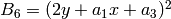and respectively (in the notation of Mazur/Tate).
• x - optional ring element to use as the “x” variable. If x is None, then a new polynomial ring will be constructed over the base ring of the elliptic curve, and its generator will be used as x. Note that x does not need to be a generator of a polynomial ring; any ring element is ok. This permits fast calculation of the torsion polynomial evaluated on any element of a ring.
• cache - optional dictionary, with integer keys. If the key m is in cache, then cache[m] is assumed to be the value of division_polynomial_0(m) for the supplied x. New entries will be added to the cache as they are computed.

ALGORITHM:

Recursion described in Mazur/Tate. The recursive formulae are evaluated times.

AUTHORS:

• David Harvey (2006-09-24): initial version
• John Cremona (2008-08-26): unified division polynomial code

EXAMPLES:

sage: E = EllipticCurve("37a")
sage: E.division_polynomial_0(1)
1
sage: E.division_polynomial_0(2)
1
sage: E.division_polynomial_0(3)
3*x^4 - 6*x^2 + 3*x - 1
sage: E.division_polynomial_0(4)
2*x^6 - 10*x^4 + 10*x^3 - 10*x^2 + 2*x + 1
sage: E.division_polynomial_0(5)
5*x^12 - 62*x^10 + 95*x^9 - 105*x^8 - 60*x^7 + 285*x^6 - 174*x^5 - 5*x^4 - 5*x^3 + 35*x^2 - 15*x + 2
sage: E.division_polynomial_0(6)
3*x^16 - 72*x^14 + 168*x^13 - 364*x^12 + 1120*x^10 - 1144*x^9 + 300*x^8 - 540*x^7 + 1120*x^6 - 588*x^5 - 133*x^4 + 252*x^3 - 114*x^2 + 22*x - 1
sage: E.division_polynomial_0(7)
7*x^24 - 308*x^22 + 986*x^21 - 2954*x^20 + 28*x^19 + 17171*x^18 - 23142*x^17 + 511*x^16 - 5012*x^15 + 43804*x^14 - 7140*x^13 - 96950*x^12 + 111356*x^11 - 19516*x^10 - 49707*x^9 + 40054*x^8 - 124*x^7 - 18382*x^6 + 13342*x^5 - 4816*x^4 + 1099*x^3 - 210*x^2 + 35*x - 3
sage: E.division_polynomial_0(8)
4*x^30 - 292*x^28 + 1252*x^27 - 5436*x^26 + 2340*x^25 + 39834*x^24 - 79560*x^23 + 51432*x^22 - 142896*x^21 + 451596*x^20 - 212040*x^19 - 1005316*x^18 + 1726416*x^17 - 671160*x^16 - 954924*x^15 + 1119552*x^14 + 313308*x^13 - 1502818*x^12 + 1189908*x^11 - 160152*x^10 - 399176*x^9 + 386142*x^8 - 220128*x^7 + 99558*x^6 - 33528*x^5 + 6042*x^4 + 310*x^3 - 406*x^2 + 78*x - 5

sage: E.division_polynomial_0(18) % E.division_polynomial_0(6) == 0
True

An example to illustrate the relationship with torsion points:

sage: F = GF(11)
sage: E = EllipticCurve(F, [0, 2]); E
Elliptic Curve defined by y^2  = x^3 + 2 over Finite Field of size 11
sage: f = E.division_polynomial_0(5); f
5*x^12 + x^9 + 8*x^6 + 4*x^3 + 7
sage: f.factor()
(5) * (x^2 + 5) * (x^2 + 2*x + 5) * (x^2 + 5*x + 7) * (x^2 + 7*x + 7) * (x^2 + 9*x + 5) * (x^2 + 10*x + 7)

This indicates that the x-coordinates of all the 5-torsion points of are in , and therefore the -coordinates are in :

sage: K = GF(11^4, 'a')
sage: X = E.change_ring(K)
sage: f = X.division_polynomial_0(5)
sage: x_coords = f.roots(multiplicities=False); x_coords
[10*a^3 + 4*a^2 + 5*a + 6,
 9*a^3 + 8*a^2 + 10*a + 8,
 8*a^3 + a^2 + 4*a + 10,
 8*a^3 + a^2 + 4*a + 8,
 8*a^3 + a^2 + 4*a + 4,
 6*a^3 + 9*a^2 + 3*a + 4,
 5*a^3 + 2*a^2 + 8*a + 7,
 3*a^3 + 10*a^2 + 7*a + 8,
 3*a^3 + 10*a^2 + 7*a + 3,
 3*a^3 + 10*a^2 + 7*a + 1,
 2*a^3 + 3*a^2 + a + 7,
 a^3 + 7*a^2 + 6*a]

Now we check that these are exactly the -coordinates of the 5-torsion points of :

sage: for x in x_coords:
...       assert X.lift_x(x).order() == 5

The roots of the polynomial are the -coordinates of the points such that but :

sage: E=EllipticCurve('14a1')
sage: T=E.torsion_subgroup()
sage: [n*T.0 for n in range(6)]
[(0 : 1 : 0),
(9 : 23 : 1),
(2 : 2 : 1),
(1 : -1 : 1),
(2 : -5 : 1),
(9 : -33 : 1)]
sage: pol=E.division_polynomial_0(6)
sage: xlist=pol.roots(multiplicities=False); xlist
[9, 2, -1/3, -5]
sage: [E.lift_x(x, all=True) for x in xlist]
[[(9 : 23 : 1), (9 : -33 : 1)], [(2 : 2 : 1), (2 : -5 : 1)], [], []]

Note

The point of order 2 and the identity do not appear. The points with and are not rational.

formal()

The formal group associated to this elliptic curve.

EXAMPLES:

sage: E = EllipticCurve("37a")
sage: E.formal_group()
Formal Group associated to the Elliptic Curve defined by y^2 + y = x^3 - x over Rational Field

formal_group()

The formal group associated to this elliptic curve.

EXAMPLES:

sage: E = EllipticCurve("37a")
sage: E.formal_group()
Formal Group associated to the Elliptic Curve defined by y^2 + y = x^3 - x over Rational Field

gen(i)

Function returning the i’th generator of this elliptic curve.

Note

Relies on gens() being implemented.

EXAMPLES:

sage: R.<a1,a2,a3,a4,a6>=QQ[]
sage: E=EllipticCurve([a1,a2,a3,a4,a6])
sage: E.gen(0)
...
NotImplementedError: not implemented.

gens()

Placeholder function to return generators of an elliptic curve.

Note

This functionality is implemented in certain derived classes, such as EllipticCurve_rational_field.

EXAMPLES:

sage: R.<a1,a2,a3,a4,a6>=QQ[]
sage: E=EllipticCurve([a1,a2,a3,a4,a6])
sage: E.gens()
...
NotImplementedError: not implemented.
sage: E=EllipticCurve(QQ,[1,1])
sage: E.gens()
[(0 : 1 : 1)]

hyperelliptic_polynomials()

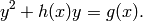
Returns a pair of polynomials , such that this elliptic curve can be defined by the standard hyperelliptic equation

EXAMPLES:

sage: R.<a1,a2,a3,a4,a6>=QQ[]
sage: E=EllipticCurve([a1,a2,a3,a4,a6])
sage: E.hyperelliptic_polynomials()
(x^3 + a2*x^2 + a4*x + a6, a1*x + a3)

is_isomorphic(other, field=None)

Returns whether or not self is isomorphic to other.

INPUT:

• other – another elliptic curve.
• field (default None) – a field into which the coefficients of the curves may be coerced (by default, uses the base field of the curves).

OUTPUT:

(bool) True if there is an isomorphism from curve self to curve other defined over field.

EXAMPLES:

sage: E = EllipticCurve('389a')
sage: F = E.change_weierstrass_model([2,3,4,5]); F
Elliptic Curve defined by y^2 + 4*x*y + 11/8*y = x^3 - 3/2*x^2 - 13/16*x over Rational Field
sage: E.is_isomorphic(F)
True
sage: E.is_isomorphic(F.change_ring(CC))
False

is_on_curve(x, y)

Returns True if is an affine point on this curve.

INPUT:

• x, y - elements of the base ring of the curve.

EXAMPLES:

sage: E=EllipticCurve(QQ,[1,1])
sage: E.is_on_curve(0,1)
True
sage: E.is_on_curve(1,1)
False

is_x_coord(x)

Returns True if x is the -coordinate of a point on this curve.

Note

See also lift_x() to find the point(s) with a given -coordinate. This function may be useful in cases where testing an element of the base field for being a square is faster than finding its square root.

EXAMPLES:

sage: E = EllipticCurve('37a'); E
Elliptic Curve defined by y^2 + y = x^3 - x over Rational Field
sage: E.is_x_coord(1)
True
sage: E.is_x_coord(2)
True

There are no rational points with x-coordinate 3:

sage: E.is_x_coord(3)
False

However, there are such points in :

sage: E.change_ring(RR).is_x_coord(3)
True

And of course it always works in :

sage: E.change_ring(RR).is_x_coord(-3)
False
sage: E.change_ring(CC).is_x_coord(-3)
True

AUTHORS:

• John Cremona (2008-08-07): adapted from lift_x()

TEST:

sage: E=EllipticCurve('5077a1')                      
sage: [x for x in srange(-10,10) if E.is_x_coord (x)]
[-3, -2, -1, 0, 1, 2, 3, 4, 8]

sage: F=GF(32,'a')
sage: E=EllipticCurve(F,[1,0,0,0,1])
sage: set([P[0] for P in E.points() if P!=E(0)]) == set([x for x in F if E.is_x_coord(x)])
True

isomorphism_to(other)

Given another weierstrass model other of self, return an isomorphism from self to other.

INPUT:

• other – an elliptic curve isomorphic to self.

OUTPUT:

(Weierstrassmorphism) An isomorphism from self to other.

Note

If the curves in question are not isomorphic, a ValueError is raised.

EXAMPLES:

sage: E = EllipticCurve('37a')
sage: F = E.short_weierstrass_model()
sage: w = E.isomorphism_to(F); w
Generic morphism:
From: Abelian group of points on Elliptic Curve defined by y^2 + y = x^3 - x over Rational Field
To:   Abelian group of points on Elliptic Curve defined by y^2  = x^3 - 16*x + 16 over Rational Field
Via:  (u,r,s,t) = (1/2, 0, 0, -1/2)
sage: P = E(0,-1,1)
sage: w(P)
(0 : -4 : 1)
sage: w(5*P)
(1 : 1 : 1)
sage: 5*w(P)
(1 : 1 : 1)
sage: 120*w(P) == w(120*P)
True

We can also handle injections to different base rings:

sage: K.<a> = NumberField(x^3-7)
sage: E.isomorphism_to(E.change_ring(K))
Generic morphism:
  From: Abelian group of points on Elliptic Curve defined by y^2 + y = x^3 - x over Rational Field
  To:   Abelian group of points on Elliptic Curve defined by y^2 + y = x^3 + (-1)*x over Number Field in a with defining polynomial x^3 - 7
  Via:  (u,r,s,t) = (1, 0, 0, 0)

isomorphisms(other, field=None)

Return the set of isomorphisms from self to other (as a list).

INPUT:

• other – another elliptic curve.
• field (default None) – a field into which the coefficients of the curves may be coerced (by default, uses the base field of the curves).

OUTPUT:

(list) A list of WeierstrassIsomorphism objects consisting of all the isomorphisms from the curve self to the curve other defined over field.

EXAMPLES:

sage: E = EllipticCurve_from_j(QQ(0)) # a curve with j=0 over QQ
sage: F = EllipticCurve('27a3') # should be the same one
sage: E.isomorphisms(F);       
[Generic morphism:
From: Abelian group of points on Elliptic Curve defined by y^2 + y = x^3 over Rational Field
To:   Abelian group of points on Elliptic Curve defined by y^2 + y = x^3 over Rational Field
Via:  (u,r,s,t) = (-1, 0, 0, -1), Generic morphism:
From: Abelian group of points on Elliptic Curve defined by y^2 + y = x^3 over Rational Field
To:   Abelian group of points on Elliptic Curve defined by y^2 + y = x^3 over Rational Field
Via:  (u,r,s,t) = (1, 0, 0, 0)]

We can also find isomorphisms defined over extension fields:

sage: E=EllipticCurve(GF(7),[0,0,0,1,1])
sage: F=EllipticCurve(GF(7),[0,0,0,1,-1])
sage: E.isomorphisms(F)
[]
sage: E.isomorphisms(F,GF(49,'a'))
[Generic morphism:
From: Abelian group of points on Elliptic Curve defined by y^2 = x^3 + x + 1 over Finite Field in a of size 7^2
To:   Abelian group of points on Elliptic Curve defined by y^2 = x^3 + x + 6 over Finite Field in a of size 7^2
Via:  (u,r,s,t) = (a + 3, 0, 0, 0), Generic morphism:
From: Abelian group of points on Elliptic Curve defined by y^2 = x^3 + x + 1 over Finite Field in a of size 7^2
To:   Abelian group of points on Elliptic Curve defined by y^2 = x^3 + x + 6 over Finite Field in a of size 7^2
Via:  (u,r,s,t) = (6*a + 4, 0, 0, 0)]

j_invariant()

Returns the j-invariant of this elliptic curve.

EXAMPLES:

sage: E = EllipticCurve([0,0,1,-1,0])
sage: E.j_invariant()
110592/37
sage: E = EllipticCurve([0, -1, 1, -10, -20])
sage: E.j_invariant()
-122023936/161051
sage: E = EllipticCurve([-4,0])
sage: E.j_invariant()
1728

sage: E = EllipticCurve([GF(7)(2),1])
sage: E.j_invariant()
1

lift_x(x, all=False)

Returns one or all points with given -coordinate.

INPUT:

• x – an element of the base ring of the curve.
• all (bool, default False) – if True, return a (possibly empty) list of all points; if False, return just one point, or raise a ValueError if there are none.

Note

See also is_x_coord().

EXAMPLES:

sage: E = EllipticCurve('37a'); E
Elliptic Curve defined by y^2 + y = x^3 - x over Rational Field
sage: E.lift_x(1)
(1 : 0 : 1)
sage: E.lift_x(2)
(2 : 2 : 1)
sage: E.lift_x(1/4, all=True)
[(1/4 : -3/8 : 1), (1/4 : -5/8 : 1)]

There are no rational points with -coordinate 3:

sage: E.lift_x(3)
...
ValueError: No point with x-coordinate 3 on Elliptic Curve defined by y^2 + y = x^3 - x over Rational Field

However, there are two such points in :

sage: E.change_ring(RR).lift_x(3, all=True)
[(3.00000000000000 : 4.42442890089805 : 1.00000000000000), (3.00000000000000 : -5.42442890089805 : 1.00000000000000)]

And of course it always works in :

sage: E.change_ring(RR).lift_x(.5, all=True)
[]
sage: E.change_ring(CC).lift_x(.5)
(0.500000000000000 : -0.500000000000000 + 0.353553390593274*I : 1.00000000000000)

We can perform these operations over finite fields too:

sage: E = E.change_ring(GF(17)); E
Elliptic Curve defined by y^2 + y = x^3 + 16*x over Finite Field of size 17
sage: E.lift_x(7)
(7 : 11 : 1)
sage: E.lift_x(3)
...
ValueError: No point with x-coordinate 3 on Elliptic Curve defined by y^2 + y = x^3 + 16*x over Finite Field of size 17

Note that there is only one lift with -coordinate 10 in :

sage: E.lift_x(10, all=True)
[(10 : 8 : 1)]

We can lift over more exotic rings too:

sage: E = EllipticCurve('37a');
sage: E.lift_x(pAdicField(17, 5)(6))
(6 + O(17^5) : 2 + 16*17 + 16*17^2 + 16*17^3 + 16*17^4 + O(17^5) : 1 + O(17^5))
sage: K.<t> = PowerSeriesRing(QQ, 't', 5)
sage: E.lift_x(1+t)
(1 + t : 2*t - t^2 + 5*t^3 - 21*t^4 + O(t^5) : 1)
sage: K.<a> = GF(16)
sage: E = E.change_ring(K)
sage: E.lift_x(a^3)
(a^3 : a^3 + a : 1)

AUTHOR:

• Robert Bradshaw (2007-04-24)

TEST:

sage: E = EllipticCurve('37a').short_weierstrass_model().change_ring(GF(17))
sage: E.lift_x(3, all=True)
[]
sage: E.lift_x(7, all=True)
[(7 : 3 : 1), (7 : 14 : 1)]

multiplication_by_m(m, x_only=False)

Return the multiplication-by- map from self to self as a pair of rational functions in two variables ,`y`.

INPUT:

• m - a nonzero integer
• x_only - bool (default: False) if True, return only the -coordinate of the map.

OUTPUT:

(2-tuple) , where and are rational functions with the degree of in exactly 1.

EXAMPLES:

sage: E = EllipticCurve([-1,3])

We verify that multiplication by 1 is just the identity:

sage: E.multiplication_by_m(1)
(x, y)

Multiplication by 2 is more complicated:

sage: f = E.multiplication_by_m(2)
sage: f
((x^4 + 2*x^2 - 24*x + 1)/(4*x^3 - 4*x + 12), (8*x^6*y - 40*x^4*y + 480*x^3*y - 40*x^2*y + 96*x*y - 568*y)/(64*x^6 - 128*x^4 + 384*x^3 + 64*x^2 - 384*x + 576))

Grab only the x-coordinate (less work):

sage: E.multiplication_by_m(2, x_only=True)
(x^4 + 2*x^2 - 24*x + 1)/(4*x^3 - 4*x + 12)

We check that it works on a point:

sage: P = E([2,3])
sage: eval = lambda f,P: [fi(P[0],P[1]) for fi in f]
sage: assert E(eval(f,P)) == 2*P

We do the same but with multiplication by 3:

sage: f = E.multiplication_by_m(3)
sage: assert E(eval(f,P)) == 3*P

And the same with multiplication by 4:

sage: f = E.multiplication_by_m(4)
sage: assert E(eval(f,P)) == 4*P

And the same with multiplication by -1,-2,-3,-4:

sage: for m in [-1,-2,-3,-4]:
...       f = E.multiplication_by_m(m)
...       assert E(eval(f,P)) == m*P

TESTS:

Verify for this fairly random looking curve and point that multiplication by m returns the right result for the first 10 integers:

sage: E = EllipticCurve([23,-105])
sage: P = E([129/4, 1479/8])
sage: for n in [1..10]:
...       f = E.multiplication_by_m(n)
...       Q = n*P
...       assert Q == E(eval(f,P))
...       f = E.multiplication_by_m(-n)
...       Q = -n*P
...       assert Q == E(eval(f,P))

The following test shows that #4364 is indeed fixed:

sage: p = next_prime(2^30-41)
sage: a = GF(p)(1)
sage: b = GF(p)(1)
sage: E = EllipticCurve([a, b])
sage: P = E.random_point()
sage: my_eval = lambda f,P: [fi(P[0],P[1]) for fi in f]
sage: f = E.multiplication_by_m(2)
sage: assert(E(eval(f,P)) == 2*P)

multiplication_by_m_isogeny(m)

Return the EllipticCurveIsogeny object associated to the multiplication-by- map on self. The resulting isogeny will have the associated rational maps (i.e. those returned by ) already computed.

NOTE: This function is currently much slower than the result of self.multiplication_by_m(), because constructing an isogeny precomputes a significant amount of information. See trac tickets #7368 and #8014 for the status of improving this situation.

INPUT:

• m - a nonzero integer

OUTPUT:

• An EllipticCurveIsogeny object associated to the multiplication-by- map on self.

EXAMPLES:

sage: E = EllipticCurve('11a1')
sage: E.multiplication_by_m_isogeny(7)
Isogeny of degree 49 from Elliptic Curve defined by y^2 + y = x^3 - x^2 - 10*x - 20 over Rational Field to Elliptic Curve defined by y^2 + y = x^3 - x^2 - 10*x - 20 over Rational Field

pari_curve(prec=53)

Return the PARI curve corresponding to this elliptic curve.

Note

The result is cached; on subsequent calls the cached value is returned provided that it has sufficient precision, otherwise pari is called again with the new precision.

EXAMPLES:

sage: E = EllipticCurve([RR(0), RR(0), RR(1), RR(-1), RR(0)])
sage: e = E.pari_curve()
sage: type(e)
<type 'sage.libs.pari.gen.gen'>
sage: e.type()
't_VEC'
sage: e.disc()
37.0000000000000

plot(xmin=None, xmax=None, **args)

Draw a graph of this elliptic curve.

INPUT:

• xmin, xmax - (optional) points will be computed at least within this range, but possibly farther.
• **args - all other options are passed to the line graphing primitive.

EXAMPLES:

sage: E = EllipticCurve([0,-1])
sage: plot(E, rgbcolor=hue(0.7))
sage: E = EllipticCurve('37a')
sage: plot(E)
sage: plot(E, xmin=25,xmax=25)

rst_transform(r, s, t)

Returns the transform of the curve by (with ).

INPUT:

• r, s, t – three elements of the base ring.

OUTPUT:

The elliptic curve obtained from self by the standard Weierstrass transformation with .

Note

This is just a special case of change_weierstrass_model(), with .

EXAMPLES:

sage: R.<r,s,t>=QQ[]
sage: E=EllipticCurve([1,2,3,4,5])
sage: E.rst_transform(r,s,t)
Elliptic Curve defined by y^2 + (2*s+1)*x*y + (r+2*t+3)*y = x^3 + (-s^2+3*r-s+2)*x^2 + (3*r^2-r*s-2*s*t+4*r-3*s-t+4)*x + (r^3+2*r^2-r*t-t^2+4*r-3*t+5) over Multivariate Polynomial Ring in r, s, t over Rational Field

scale_curve(u)

Returns the transform of the curve by scale factor .

INPUT:

• u – an invertible element of the base ring.

OUTPUT:

The elliptic curve obtained from self by the standard Weierstrass transformation with .

Note

This is just a special case of change_weierstrass_model(), with .

EXAMPLES:

sage: K=Frac(PolynomialRing(QQ,'u'))
sage: u=K.gen()
sage: E=EllipticCurve([1,2,3,4,5])       
sage: E.scale_curve(u)
Elliptic Curve defined by y^2 + u*x*y + 3*u^3*y = x^3 + 2*u^2*x^2 + 4*u^4*x + 5*u^6 over Fraction Field of Univariate Polynomial Ring in u over Rational Field

short_weierstrass_model(complete_cube=True)

Returns a short Weierstrass model for self.

INPUT:

• complete_cube - bool (default: True); for meaning, see below.

OUTPUT:

An elliptic curve.

If complete_cube=True: Return a model of the form for this curve. The characteristic must not be 2; in characteristic 3, it is only possible if .

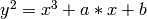
If complete_cube=False: Return a model of the form for this curve. The characteristic must not be 2.

EXAMPLES:

sage: E = EllipticCurve([1,2,3,4,5])
sage: print E
Elliptic Curve defined by y^2 + x*y + 3*y = x^3 + 2*x^2 + 4*x + 5 over Rational Field
sage: F = E.short_weierstrass_model()
sage: print F
Elliptic Curve defined by y^2  = x^3 + 4941*x + 185166 over Rational Field
sage: E.is_isomorphic(F)
True
sage: F = E.short_weierstrass_model(complete_cube=False)
sage: print F
Elliptic Curve defined by y^2  = x^3 + 9*x^2 + 88*x + 464 over Rational Field
sage: print E.is_isomorphic(F)
True

sage: E = EllipticCurve(GF(3),[1,2,3,4,5])
sage: E.short_weierstrass_model(complete_cube=False)
Elliptic Curve defined by y^2 = x^3 + x + 2 over Finite Field of size 3

This used to be different see trac #3973:

sage: E.short_weierstrass_model()
Elliptic Curve defined by y^2 = x^3 + x + 2 over Finite Field of size 3

More tests in characteristic 3:

sage: E = EllipticCurve(GF(3),[0,2,1,2,1])
sage: E.short_weierstrass_model()
...
ValueError: short_weierstrass_model(): no short model for Elliptic Curve defined by y^2 + y = x^3 + 2*x^2 + 2*x + 1 over Finite Field of size 3 (characteristic is 3)
sage: E.short_weierstrass_model(complete_cube=False)
Elliptic Curve defined by y^2 = x^3 + 2*x^2 + 2*x + 2 over Finite Field of size 3
sage: E.short_weierstrass_model(complete_cube=False).is_isomorphic(E)
True

torsion_polynomial(m, x=None, two_torsion_multiplicity=2)

Returns the division polynomial of this elliptic curve evaluated at x.

INPUT:

• m - positive integer.

• x - optional ring element to use as the “x” variable. If x is None, then a new polynomial ring will be constructed over the base ring of the elliptic curve, and its generator will be used as x. Note that x does not need to be a generator of a polynomial ring; any ring element is ok. This permits fast calculation of the torsion polynomial evaluated on any element of a ring.

• two_torsion_multiplicity - 0,1 or 2

  If 0: for even when x is None, a univariate polynomial over the base ring of the curve is returned, which omits factors whose roots are the -coordinates of the -torsion points. Similarly when is not none, the evaluation of such a polynomial at is returned.

  If 2: for even when x is None, a univariate polynomial over the base ring of the curve is returned, which includes a factor of degree 3 whose roots are the -coordinates of the -torsion points. Similarly when is not none, the evaluation of such a polynomial at is returned.

  If 1: when x is None, a bivariate polynomial over the base ring of the curve is returned, which includes a factor which has simple zeros at the -torsion points. When is not none, it should be a tuple of length 2, and the evaluation of such a polynomial at is returned.

EXAMPLES:

sage: E = EllipticCurve([0,0,1,-1,0])
sage: E.division_polynomial(1)
1
sage: E.division_polynomial(2, two_torsion_multiplicity=0)
1
sage: E.division_polynomial(2, two_torsion_multiplicity=1)
2*y + 1
sage: E.division_polynomial(2, two_torsion_multiplicity=2)
4*x^3 - 4*x + 1
sage: E.division_polynomial(2)
4*x^3 - 4*x + 1
sage: [E.division_polynomial(3, two_torsion_multiplicity=i) for i in range(3)]
[3*x^4 - 6*x^2 + 3*x - 1, 3*x^4 - 6*x^2 + 3*x - 1, 3*x^4 - 6*x^2 + 3*x - 1]
sage: [type(E.division_polynomial(3, two_torsion_multiplicity=i)) for i in range(3)]
[<class 'sage.rings.polynomial.polynomial_element_generic.Polynomial_rational_dense'>,
<type 'sage.rings.polynomial.multi_polynomial_libsingular.MPolynomial_libsingular'>,
<class 'sage.rings.polynomial.polynomial_element_generic.Polynomial_rational_dense'>]

sage: E = EllipticCurve([0, -1, 1, -10, -20]) 
sage: R.<z>=PolynomialRing(QQ)               
sage: E.division_polynomial(4,z,0)
2*z^6 - 4*z^5 - 100*z^4 - 790*z^3 - 210*z^2 - 1496*z - 5821
sage: E.division_polynomial(4,z)                           
8*z^9 - 24*z^8 - 464*z^7 - 2758*z^6 + 6636*z^5 + 34356*z^4 + 53510*z^3 + 99714*z^2 + 351024*z + 459859

This does not work, since when two_torsion_multiplicity is 1, we compute a bivariate polynomial, and must evaluate at a tuple of length 2:

sage: E.division_polynomial(4,z,1)
...
ValueError: x should be a tuple of length 2 (or None) when two_torsion_multiplicity is 1
sage: R.<z,w>=PolynomialRing(QQ,2)               
sage: E.division_polynomial(4,(z,w),1).factor()
(2*w + 1) * (2*z^6 - 4*z^5 - 100*z^4 - 790*z^3 - 210*z^2 - 1496*z - 5821)       

We can also evaluate this bivariate polynomial at a point:

sage: P = E(5,5)
sage: E.division_polynomial(4,P,two_torsion_multiplicity=1)
-1771561

two_division_polynomial(x=None)

Returns the 2-division polynomial of this elliptic curve evaluated at x.

INPUT:

• x - optional ring element to use as the variable. If x is None, then a new polynomial ring will be constructed over the base ring of the elliptic curve, and its generator will be used as x. Note that x does not need to be a generator of a polynomial ring; any ring element is ok. This permits fast calculation of the torsion polynomial evaluated on any element of a ring.

EXAMPLES:

sage: E=EllipticCurve('5077a1')
sage: E.two_division_polynomial()
4*x^3 - 28*x + 25
sage: E=EllipticCurve(GF(3^2,'a'),[1,1,1,1,1])
sage: E.two_division_polynomial()          
x^3 + 2*x^2 + 2
sage: E.two_division_polynomial().roots()  
[(2, 1), (2*a, 1), (a + 2, 1)]

sage.schemes.elliptic_curves.ell_generic.is_EllipticCurve(x)

Utility function to test if x is an instance of an Elliptic Curve class.

EXAMPLES:

sage: from sage.schemes.elliptic_curves.ell_generic import is_EllipticCurve
sage: E = EllipticCurve([1,2,3/4,7,19])
sage: is_EllipticCurve(E)
True
sage: is_EllipticCurve(0)
False