AUTHORS:
This module provides easy access to many of Maxima and PARI’s special functions.
Maxima’s special functions package (which includes spherical harmonic functions, spherical Bessel functions (of the 1st and 2nd kind), and spherical Hankel functions (of the 1st and 2nd kind)) was written by Barton Willis of the University of Nebraska at Kearney. It is released under the terms of the General Public License (GPL).
Support for elliptic functions and integrals was written by Raymond Toy. It is placed under the terms of the General Public License (GPL) that governs the distribution of Maxima.
The (usual) Bessel functions and Airy functions are part of the
standard Maxima package. Some Bessel functions also are implemented
in Pari. (Caution: The Pari versions are sometimes different than
the Maxima version.) For example, the K-Bessel function
 can be computed using either Maxima or Pari,
depending on an optional variable you pass to bessel_K.
can be computed using either Maxima or Pari,
depending on an optional variable you pass to bessel_K.
Next, we summarize some of the properties of the functions implemented here.
Bessel functions, first defined by the Swiss mathematician Daniel Bernoulli and named after Friedrich Bessel, are canonical solutions y(x) of Bessel’s differential equation:
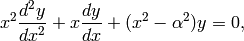
for an arbitrary real number  (the order).
Another important formulation of the two linearly independent
solutions to Bessel’s equation are the Hankel functions
 and
and  ,
defined by:
,
defined by:
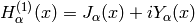
where  is the imaginary unit (and
  and
and
 are the usual J- and Y-Bessel functions). These
linear combinations are also known as Bessel functions of the third
kind; they are two linearly independent solutions of Bessel’s
differential equation. They are named for Hermann Hankel.
are the usual J- and Y-Bessel functions). These
linear combinations are also known as Bessel functions of the third
kind; they are two linearly independent solutions of Bessel’s
differential equation. They are named for Hermann Hankel.
Airy function The function  and the related
function
and the related
function  , which is also called an Airy function,
are solutions to the differential equation
, which is also called an Airy function,
are solutions to the differential equation

known as the Airy equation. They belong to the class of ‘Bessel functions of
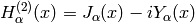
fractional order’. The initial conditions
 ,
,
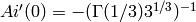 define
. The initial conditions
define
. The initial conditions
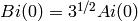 ,
, 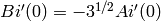 define .
They are named after the British astronomer George Biddell Airy.
Spherical harmonics: Laplace’s equation in spherical coordinates is:
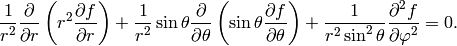
Note that the spherical coordinates  and
and
 are defined here as follows: is
the colatitude or polar angle, ranging from
are defined here as follows: is
the colatitude or polar angle, ranging from
 and the azimuth or
longitude, ranging from
and the azimuth or
longitude, ranging from  .
.
The general solution which remains finite towards infinity is a linear combination of functions of the form
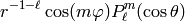
and
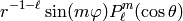
where  are the associated Legendre polynomials,
and with integer parameters
are the associated Legendre polynomials,
and with integer parameters  and
and  from
from  to
to  . Put in another way, the
solutions with integer parameters and
. Put in another way, the
solutions with integer parameters and
 , can be written as linear
combinations of:
, can be written as linear
combinations of:
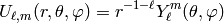
where the functions  are the spherical harmonic
functions with parameters , , which can be
written as:
are the spherical harmonic
functions with parameters , , which can be
written as:
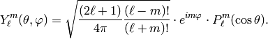
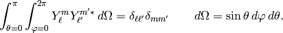
The spherical harmonics obey the normalisation condition
When solving for separable solutions of Laplace’s equation in spherical coordinates, the radial equation has the form:
![x^2 \frac{d^2 y}{dx^2} + 2x \frac{dy}{dx} + [x^2 - n(n+1)]y = 0.](../../_images/math/55d1814a562cc9232c15bfaf811a397ca6b2bde7.png)
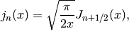
The spherical Bessel functions  and
and  ,
are two linearly independent solutions to this equation. They are
related to the ordinary Bessel functions
,
are two linearly independent solutions to this equation. They are
related to the ordinary Bessel functions  and
and
 by:
by:
For  , the confluent hypergeometric function
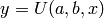 is defined to be the solution to Kummer’s
differential equation
is defined to be the solution to Kummer’s
differential equation

which satisfies 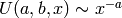 , as
, as
 . (There is a linearly independent
solution, called Kummer’s function
. (There is a linearly independent
solution, called Kummer’s function  , which is not
implemented.)
, which is not
implemented.)
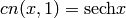
Jacobi elliptic functions can be thought of as generalizations of both ordinary and hyperbolic trig functions. There are twelve Jacobian elliptic functions. Each of the twelve corresponds to an arrow drawn from one corner of a rectangle to another.
n ------------------- d
|                     |
|                     |
|                     |
s ------------------- c
Each of the corners of the rectangle are labeled, by convention, s, c, d and n. The rectangle is understood to be lying on the complex plane, so that s is at the origin, c is on the real axis, and n is on the imaginary axis. The twelve Jacobian elliptic functions are then pq(x), where p and q are one of the letters s,c,d,n.
The Jacobian elliptic functions are then the unique doubly-periodic, meromorphic functions satisfying the following three properties:
We can write
where  ,
,  , and
, and  are any of the
letters
are any of the
letters  ,
,  ,
,  ,
,  , with
the understanding that
, with
the understanding that  .
.
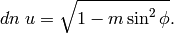
Let
Then the Jacobi elliptic function  is given by

and  is given by

and
To emphasize the dependence on , one can write
 for example (and similarly for
  and
and
 ). This is the notation used below.
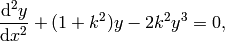
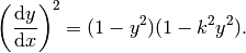
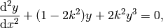
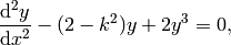
For a given  with
with  they therefore are
solutions to the following nonlinear ordinary differential
equations:
they therefore are
solutions to the following nonlinear ordinary differential
equations:
 solves the differential equations
and
 solves the differential equations
and 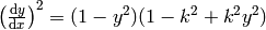 .
.
 solves the differential equations
and 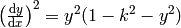 .
.
If  denotes the complete elliptic integral of the
first kind (denoted elliptic_kc), the elliptic functions
denotes the complete elliptic integral of the
first kind (denoted elliptic_kc), the elliptic functions
 and
and  have real periods
 , whereas
  has a period
 . The limit
  gives
gives
 and trigonometric functions:
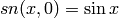 ,
, 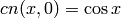 ,
,
 . The limit
  gives
gives
 and hyperbolic functions:
 ,
,
 ,
,
 .
.
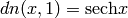
The incomplete elliptic integrals (of the first kind, etc.) are:
and the complete ones are obtained by taking  .
.
REFERENCES:
TODO: Resolve weird bug in commented out code in hypergeometric_U below.
AUTHORS:
Added 16-02-2008 (wdj): optional calls to scipy and replace all ‘#random’ by ‘...’ (both at the request of William Stein)
Warning
SciPy’s versions are poorly documented and seem less accurate than the Maxima and Pari versions.
A class implementing the I, J, K, and Y Bessel functions.
EXAMPLES:
sage: g = Bessel(2); g
J_{2}
sage: print g
J-Bessel function of order 2
sage: g.plot(0,10)
Returns the order of this Bessel function.
TEST:
sage: a = Bessel(3,'K')
sage: a.order()
3
Enables easy plotting of all the Bessel functions directly from the Bessel class.
TESTS:
sage: plot(Bessel(2),3,4)
sage: Bessel(2).plot(3,4)
sage: P = Bessel(2,'I').plot(1,5)
sage: P += Bessel(2,'J').plot(1,5)
sage: P += Bessel(2,'K').plot(1,5)
sage: P += Bessel(2,'Y',algorithm='maxima').plot(1,5) # default algorithm Pari not available for this one
sage: show(P)
Returns the precision (in number of bits) used to represent this Bessel function.
TESTS:
sage: a = Bessel(3,'K')
sage: a.prec()
53
sage: B = Bessel(20,prec=100); B
J_{20}
sage: B.prec()
100
Returns the package used, e.g. Maxima, Pari, or SciPy, to compute with this Bessel function.
TESTS:
sage: Bessel(20,algorithm='maxima').system()
'maxima'
sage: Bessel(20,prec=100).system()
'pari'
Returns the type of this Bessel object.
TEST:
sage: a = Bessel(3,'K')
sage: a.type()
'K'
Bases: sage.functions.special.MaximaFunction
This returns the value of the “incomplete elliptic integral of the second kind,”
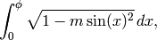
i.e., integrate(sqrt(1 - m*sin(x)^2), x, 0, phi). Taking  gives elliptic_ec.
EXAMPLES:
sage: z = var("z")
sage: elliptic_e(z, 1)
sin(z)
sage: elliptic_e(z, 0)
z
sage: elliptic_e(0.5, 0.1)
0.498011394499

sage: loads(dumps(elliptic_e))
elliptic_e
Bases: sage.functions.special.MaximaFunction
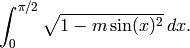
This returns the value of the “complete elliptic integral of the second kind,”
EXAMPLES:
sage: elliptic_ec(0.1)
1.5307576369
sage: elliptic_ec(x).diff()
1/2*(elliptic_ec(x) - elliptic_kc(x))/x

sage: loads(dumps(elliptic_ec))
elliptic_ec
Bases: sage.functions.special.MaximaFunction
This returns the value of the “incomplete elliptic integral of the second kind,”
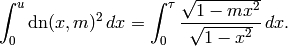
where  .
.
EXAMPLES:
sage: elliptic_eu (0.5, 0.1)
0.496054551287
Bases: sage.functions.special.MaximaFunction
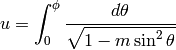
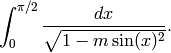
This returns the value of the “incomplete elliptic integral of the first kind,”
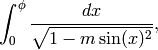
i.e., integrate(1/sqrt(1 - m*sin(x)^2), x, 0, phi). Taking
 gives elliptic_kc.
EXAMPLES:
sage: z = var("z")
sage: elliptic_f (z, 0)
z
sage: elliptic_f (z, 1)
log(tan(1/4*pi + 1/2*z))
sage: elliptic_f (0.2, 0.1)
0.200132506748
Bases: sage.functions.special.MaximaFunction
This returns the value of the “complete elliptic integral of the first kind,”
EXAMPLES:
sage: elliptic_kc(0.5)
1.8540746773
sage: elliptic_f(RR(pi/2), 0.5)
1.8540746773
Bases: sage.functions.special.MaximaFunction
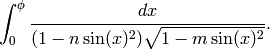
This returns the value of the “incomplete elliptic integral of the third kind,”
EXAMPLES:
sage: elliptic_pi(0.1, 0.2, 0.3)
0.200665068221
Bases: sage.symbolic.function.BuiltinFunction
EXAMPLES:
sage: from sage.functions.special import MaximaFunction
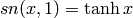
sage: f = MaximaFunction("jacobi_sn")
sage: f(1,1)
tanh(1)
sage: f(1/2,1/2).n()
0.470750473655657
The function and the related function ,
which is also called an Airy function, are
solutions to the differential equation

known as the Airy equation. The initial conditions
,
define .
The initial conditions ,
define .
They are named after the British astronomer George Biddell Airy. They belong to the class of “Bessel functions of fractional order”.
EXAMPLES:
sage: airy_ai(1.0)        # last few digits are random
0.135292416312881400
sage: airy_bi(1.0)        # last few digits are random
1.20742359495287099
REFERENCE:
The function and the related function ,
which is also called an Airy function, are
solutions to the differential equation
known as the Airy equation. The initial conditions
,
define .
The initial conditions ,
define .
They are named after the British astronomer George Biddell Airy. They belong to the class of “Bessel functions of fractional order”.
EXAMPLES:
sage: airy_ai(1)        # last few digits are random
0.135292416312881400
sage: airy_bi(1)        # last few digits are random
1.20742359495287099
REFERENCE:
Implements the “I-Bessel function”, or “modified Bessel function, 1st kind”, with index (or “order”) nu and argument z.
INPUT:
DEFINITION:
Maxima:
                 inf
                ====   - nu - 2 k  nu + 2 k
                \     2          z
                 >    -------------------
                /     k! Gamma(nu + k + 1)
                ====
                k = 0

Pari:

                 inf
                ====   - 2 k  2 k
                \     2      z    Gamma(nu + 1)
                 >    -----------------------
                /       k! Gamma(nu + k + 1)
                ====
                k = 0
Sometimes bessel_I(nu,z) is denoted I_nu(z) in the literature.
Warning
In Maxima (the manual says) i0 is deprecated but bessel_i(0,*) is broken. (Was fixed in recent CVS patch though.)
EXAMPLES:
sage: bessel_I(1,1,"pari",500)
0.565159103992485027207696027609863307328899621621092009480294489479255640964371134092664997766814410064677886055526302676857637684917179812041131208121
sage: bessel_I(1,1)
0.565159103992485
sage: bessel_I(2,1.1,"maxima")
0.16708949925104...
sage: bessel_I(0,1.1,"maxima")
1.32616018371265...
sage: bessel_I(0,1,"maxima")
1.2660658777520...
sage: bessel_I(1,1,"scipy")
0.565159103992...
Return value of the “J-Bessel function”, or “Bessel function, 1st kind”, with index (or “order”) nu and argument z.
Defn:
Maxima:
                 inf
                ====          - nu - 2 k  nu + 2 k
                \     (-1)^k 2           z
                 >    -------------------------
                /        k! Gamma(nu + k + 1)
                ====
                k = 0

Pari:

                 inf
                ====          - 2k    2k
                \     (-1)^k 2      z    Gamma(nu + 1)
                 >    ----------------------------
                /         k! Gamma(nu + k + 1)
                ====
                k = 0
Sometimes bessel_J(nu,z) is denoted J_nu(z) in the literature.
Warning
Inaccurate for small values of z.
EXAMPLES:
sage: bessel_J(2,1.1)
0.136564153956658
sage: bessel_J(0,1.1)
0.719622018527511
sage: bessel_J(0,1)
0.765197686557967
sage: bessel_J(0,0)
1.00000000000000
sage: bessel_J(0.1,0.1)
0.777264368097005
We check consistency of PARI and Maxima:
sage: n(bessel_J(3,10,"maxima"))
0.0583793793051...
sage: n(bessel_J(3,10,"pari"))
0.0583793793051868
sage: bessel_J(3,10,"scipy")
0.0583793793052...
Implements the “K-Bessel function”, or “modified Bessel function, 2nd kind”, with index (or “order”) nu and argument z. Defn:
 pi*(bessel_I(-nu, z) - bessel_I(nu, z))
----------------------------------------
             2*sin(pi*nu)
if nu is not an integer and by taking a limit otherwise.
Sometimes bessel_K(nu,z) is denoted K_nu(z) in the literature. In Pari, nu can be complex and z must be real and positive.
EXAMPLES:
sage: bessel_K(3,2,"scipy")
0.64738539094...
sage: bessel_K(3,2)
0.64738539094...
sage: bessel_K(1,1)
0.60190723019...
sage: bessel_K(1,1,"pari",10)
0.60
sage: bessel_K(1,1,"pari",100)
0.60190723019723457473754000154
Implements the “Y-Bessel function”, or “Bessel function of the 2nd kind”, with index (or “order”) nu and argument z.
Note
Currently only prec=53 is supported.
Defn:
 cos(pi n)*bessel_J(nu, z) - bessel_J(-nu, z)
-------------------------------------------------
                  sin(nu*pi)
if nu is not an integer and by taking a limit otherwise.
Sometimes bessel_Y(n,z) is denoted Y_n(z) in the literature.
This is computed using Maxima by default.
EXAMPLES:
sage: bessel_Y(2,1.1,"scipy")
-1.4314714939...
sage: bessel_Y(2,1.1)
-1.4314714939590...
sage: bessel_Y(3.001,2.1)
-1.0299574976424...
Note
Adding ‘0’+ inside sage_eval as a temporary bug work-around.
Returns the elliptic modular  -function evaluated at
  .
.
INPUT:
OUTPUT:
(complex) The value of  .
.
ALGORITHM:
Calls the pari function ellj().
AUTHOR:
John Cremona
EXAMPLES:
sage: elliptic_j(CC(i))
1728.00000000000
sage: elliptic_j(sqrt(-2.0))
8000.00000000000
sage: z = ComplexField(100)(1,sqrt(11))/2
sage: elliptic_j(z)
-32768.000...
sage: elliptic_j(z).real().round()
-32768
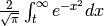
The complementary error function
 (t belongs
to RR). This function is currently always
evaluated immediately.
(t belongs
to RR). This function is currently always
evaluated immediately.
EXAMPLES:
sage: error_fcn(6)
2.15197367124989e-17
sage: error_fcn(RealField(100)(1/2))
0.47950012218695346231725334611
Note this is literally equal to  :
:
sage: 1 - error_fcn(0.5)
0.520499877813047
sage: erf(0.5)
0.520499877813047
The exponential integral  (t
belongs to RR). This function is deprecated - please use
Ei or exponential_integral_1 as needed instead.
(t
belongs to RR). This function is deprecated - please use
Ei or exponential_integral_1 as needed instead.
EXAMPLES:
sage: exp_int(6)
doctest:...: DeprecationWarning: The method expint() is deprecated. Use -Ei(-x) or exponential_integral_1(x) as needed instead.
0.000360082452162659
Default is a wrap of Pari’s hyperu(alpha,beta,x) function. Optionally, algorithm = “scipy” can be used.
The confluent hypergeometric function is
defined to be the solution to Kummer’s differential equation

This satisfies , as
, and is sometimes denoted
x^{-a}2_F_0(a,1+a-b,-1/x). This is not the same as Kummer’s
 -hypergeometric function, denoted sometimes as
_1F_1(alpha,beta,x), though it satisfies the same DE that
-hypergeometric function, denoted sometimes as
_1F_1(alpha,beta,x), though it satisfies the same DE that
 does.
does.
Warning
In the literature, both are called “Kummer confluent hypergeometric” functions.
EXAMPLES:
sage: hypergeometric_U(1,1,1,"scipy")
0.596347362323...
sage: hypergeometric_U(1,1,1)
0.59634736232319...
sage: hypergeometric_U(1,1,1,"pari",70)
0.59634736232319407434...
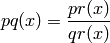
Here sym = “pq”, where p,q in c,d,n,s. This returns the value of
the inverse Jacobi function  . There are a
total of 12 functions described by this.
. There are a
total of 12 functions described by this.
EXAMPLES:
sage: jacobi("sn",1/2,1/2)
jacobi_sn(1/2, 1/2)
sage: float(jacobi("sn",1/2,1/2))
0.4707504736556572
sage: float(inverse_jacobi("sn",0.47,1/2))
0.49909823132221959
sage: float(inverse_jacobi("sn",0.4707504,0.5))
0.49999991146655481
sage: P = plot(inverse_jacobi('sn', x, 0.5), 0, 1, plot_points=20)
Now to view this, just type show(P).
Here sym = “pq”, where p,q in c,d,n,s. This returns the value of the Jacobi function pq(x,m), as described in the documentation for Sage’s “special” module. There are a total of 12 functions described by this.
EXAMPLES:
sage: jacobi("sn",1,1)
tanh(1)
sage: jacobi("cd",1,1/2)
jacobi_cd(1, 1/2)
sage: RDF(jacobi("cd",1,1/2))
0.724009721659
sage: RDF(jacobi("cn",1,1/2)); RDF(jacobi("dn",1,1/2)); RDF(jacobi("cn",1,1/2)/jacobi("dn",1,1/2))
0.595976567672
0.823161001632
0.724009721659
sage: jsn = jacobi("sn",x,1)
sage: P = plot(jsn,0,1)
To view this, type P.show().
This method is deprecated, please use log_gamma() instead.
See the log_gamma() method for documentation and examples.
EXAMPLES:
sage: lngamma(RR(6))
doctest:...: DeprecationWarning: The method lngamma() is deprecated. Use log_gamma() instead.
4.78749174278205
The principal branch of the logarithm of the Gamma function of t. This function is currently always immediately evaluated for non-symbolic input.
EXAMPLES:
sage: log_gamma(RR(6))
4.78749174278205
sage: log_gamma(6)
4.78749174278205
sage: log_gamma(pari(6))
4.78749174278205
sage: log_gamma(x)
log_gamma(x)
Returns x evaluated in Maxima, then returned to Sage. This is used to evaluate several of these special functions.
TEST:
sage: from sage.functions.special import airy_ai
sage: airy_bi(1.0)
1.20742359495
Returns the spherical Bessel function of the first kind for integers n >= 1.
Reference: AS 10.1.8 page 437 and AS 10.1.15 page 439.
EXAMPLES:
sage: spherical_bessel_J(2,x)
((3/x^2 - 1)*sin(x) - 3*cos(x)/x)/x
sage: spherical_bessel_J(1, 5.2, algorithm='scipy')
-0.12277149950007...
sage: spherical_bessel_J(1, 3, algorithm='scipy')
0.345677499762355...
Returns the spherical Bessel function of the second kind for integers n -1.
Reference: AS 10.1.9 page 437 and AS 10.1.15 page 439.
EXAMPLES:
sage: x = PolynomialRing(QQ, 'x').gen()
sage: spherical_bessel_Y(2,x)
-((3/x^2 - 1)*cos(x) + 3*sin(x)/x)/x
Returns the spherical Hankel function of the first kind for
integers  , written as a string. Reference: AS
10.1.36 page 439.
, written as a string. Reference: AS
10.1.36 page 439.
EXAMPLES:
sage: spherical_hankel1(2, x)
(I*x^2 - 3*x - 3*I)*e^(I*x)/x^3
Returns the spherical Hankel function of the second kind for
integers , written as a string. Reference: AS 10.1.17 page
439.
EXAMPLES:
sage: spherical_hankel2(2, x)
(-I*x^2 - 3*x + 3*I)*e^(-I*x)/x^3
Here I = sqrt(-1).
Returns the spherical Harmonic function of the second kind for
integers ,  . Reference:
Merzbacher 9.64.
. Reference:
Merzbacher 9.64.
EXAMPLES:
sage: x,y = var('x,y')
sage: spherical_harmonic(3,2,x,y)
1/8*sqrt(7)*sqrt(30)*e^(2*I*y)*sin(x)^2*cos(x)/sqrt(pi)
sage: spherical_harmonic(3,2,1,2)
1/8*sqrt(7)*sqrt(30)*e^(4*I)*sin(1)^2*cos(1)/sqrt(pi)
