This module wraps some of the orthogonal/special functions in the Maxima package “orthopoly”. This package was written by Barton Willis of the University of Nebraska at Kearney. It is released under the terms of the General Public License (GPL). Send Maxima-related bug reports and comments on this module to willisb@unk.edu. In your report, please include Maxima and specfun version information.
The Chebyshev polynomial of the first kind arises as a solution to the differential equation

and those of the second kind as a solution to

The Chebyshev polynomials of the first kind are defined by the recurrence relation

The Chebyshev polynomials of the second kind are defined by the recurrence relation

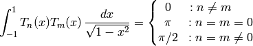
For integers  , they satisfy the orthogonality
relations
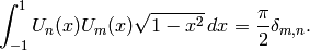
, they satisfy the orthogonality
relations
and
They are named after Pafnuty Chebyshev (alternative transliterations: Tchebyshef or Tschebyscheff).
The Hermite polynomials are defined either by
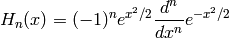
(the “probabilists’ Hermite polynomials”), or by
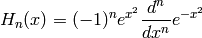
(the “physicists’ Hermite polynomials”). Sage (via Maxima) implements the latter flavor. These satisfy the orthogonality relation
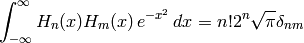
They are named in honor of Charles Hermite.
Each Legendre polynomial  is an
is an  -th degree polynomial.
It may be expressed using Rodrigues’ formula:
-th degree polynomial.
It may be expressed using Rodrigues’ formula:
![P_n(x) = (2^n n!)^{-1} {\frac{d^n}{dx^n} } \left[ (x^2 -1)^n \right].](../../_images/math/a74e6e712de4182dad842688651f5815fd0f51f0.png)
These are solutions to Legendre’s differential equation:
![{\frac{d}{dx}} \left[ (1-x^2) {\frac{d}{dx}} P(x) \right] + n(n+1)P(x) = 0.](../../_images/math/d38ec34d3bf488cd625301d8d7b724810303cb8c.png)
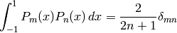
and satisfy the orthogonality relation
The Legendre function of the second kind  is another
(linearly independent) solution to the Legendre differential equation.
It is not an “orthogonal polynomial” however.
is another
(linearly independent) solution to the Legendre differential equation.
It is not an “orthogonal polynomial” however.
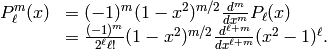
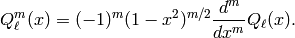
The associated Legendre functions of the first kind
 can be given in terms of the “usual”
Legendre polynomials by
can be given in terms of the “usual”
Legendre polynomials by
Assuming  , they satisfy the orthogonality
relation:
, they satisfy the orthogonality
relation:
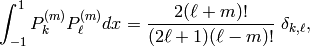
where  is the Kronecker delta.
The associated Legendre functions of the second kind
 can be given in terms of the “usual”
Legendre polynomials by
can be given in terms of the “usual”
Legendre polynomials by
They are named after Adrien-Marie Legendre.
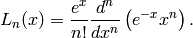
Laguerre polynomials may be defined by the Rodrigues formula
They are solutions of Laguerre’s equation:

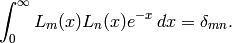
and satisfy the orthogonality relation
The generalized Laguerre polynomials may be defined by the Rodrigues formula:
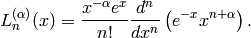
(These are also sometimes called the associated Laguerre
polynomials.) The simple Laguerre polynomials are recovered from
the generalized polynomials by setting  .
.
They are named after Edmond Laguerre.
Jacobi polynomials are a class of orthogonal polynomials. They are obtained from hypergeometric series in cases where the series is in fact finite:

where  is Pochhammer’s symbol (for the rising
factorial), (Abramowitz and Stegun p561.) and thus have the
explicit expression
is Pochhammer’s symbol (for the rising
factorial), (Abramowitz and Stegun p561.) and thus have the
explicit expression

They are named after Carl Jacobi.
Ultraspherical or Gegenbauer polynomials are given in terms of
the Jacobi polynomials  with
with
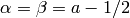 by
by
They satisfy the orthogonality relation

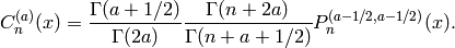
for  . They are obtained from hypergeometric series
in cases where the series is in fact finite:
. They are obtained from hypergeometric series
in cases where the series is in fact finite:
where  is the falling factorial. (See
Abramowitz and Stegun p561)
is the falling factorial. (See
Abramowitz and Stegun p561)
They are named for Leopold Gegenbauer (1849-1903).
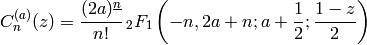
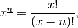
For completeness, the Pochhammer symbol, introduced by Leo August
Pochhammer,  , is used in the theory of special
functions to represent the “rising factorial” or “upper factorial”
, is used in the theory of special
functions to represent the “rising factorial” or “upper factorial”
On the other hand, the “falling factorial” or “lower factorial” is
in the notation of Ronald L. Graham, Donald E. Knuth and Oren Patashnik in their book Concrete Mathematics.
Note
The first call of any of these will usually cost a bit extra (it loads “specfun”, but I’m not sure if that is the real reason). The next call is usually faster but not always.
TODO: Implement associated Legendre polynomials and Zernike polynomials. (Neither is in Maxima.) http://en.wikipedia.org/wiki/Associated_Legendre_polynomials http://en.wikipedia.org/wiki/Zernike_polynomials
REFERENCES:
AUTHORS:
Returns the Chebyshev function of the first kind for integers
 .
.
REFERENCE:
EXAMPLES:
sage: x = PolynomialRing(QQ, 'x').gen()
sage: chebyshev_T(2,x)
2*x^2 - 1
Returns the Chebyshev function of the second kind for integers .
REFERENCE:
EXAMPLES:
sage: x = PolynomialRing(QQ, 'x').gen()
sage: chebyshev_U(2,x)
4*x^2 - 1
Returns the ultraspherical (or Gegenbauer) polynomial for integers
 .
.
Computed using Maxima.
REFERENCE:
EXAMPLES:
sage: x = PolynomialRing(QQ, 'x').gen()
sage: ultraspherical(2,3/2,x)
15/2*x^2 - 3/2
sage: ultraspherical(2,1/2,x)
3/2*x^2 - 1/2
sage: ultraspherical(1,1,x)
2*x
sage: t = PolynomialRing(RationalField(),"t").gen()
sage: gegenbauer(3,2,t)
32*t^3 - 12*t
Returns the generalized Laguerre polynomial for integers .
Typically, a = 1/2 or a = -1/2.
REFERENCE:
EXAMPLES:
sage: x = PolynomialRing(QQ, 'x').gen()
sage: gen_laguerre(2,1,x)
1/2*x^2 - 3*x + 3
sage: gen_laguerre(2,1/2,x)
1/2*x^2 - 5/2*x + 15/8
sage: gen_laguerre(2,-1/2,x)
1/2*x^2 - 3/2*x + 3/8
sage: gen_laguerre(2,0,x)
1/2*x^2 - 2*x + 1
sage: gen_laguerre(3,0,x)
-1/6*x^3 + 3/2*x^2 - 3*x + 1
Returns the generalized (or associated) Legendre function of the
first kind for integers  .
.
The awkward code for when m is odd and 1 results from the fact that
Maxima is happy with, for example,  , but
Sage is not. For these cases the function is computed from the
(m-1)-case using one of the recursions satisfied by the Legendre
functions.
, but
Sage is not. For these cases the function is computed from the
(m-1)-case using one of the recursions satisfied by the Legendre
functions.
REFERENCE:
EXAMPLES:
sage: P.<t> = QQ[]
sage: gen_legendre_P(2, 0, t)
3/2*t^2 - 1/2
sage: gen_legendre_P(2, 0, t) == legendre_P(2, t)
True
sage: gen_legendre_P(3, 1, t)
-3/2*sqrt(-t^2 + 1)*(5*t^2 - 1)
sage: gen_legendre_P(4, 3, t)
105*sqrt(-t^2 + 1)*(t^2 - 1)*t
sage: gen_legendre_P(7, 3, I).expand()
-16695*sqrt(2)
sage: gen_legendre_P(4, 1, 2.5)
-583.562373654533*I
Returns the generalized (or associated) Legendre function of the
second kind for integers ,  .
.
Maxima restricts m = n. Hence the cases m n are computed using the same recursion used for gen_legendre_P(n,m,x) when m is odd and 1.
EXAMPLES:
sage: P.<t> = QQ[]
sage: gen_legendre_Q(2,0,t)
3/4*t^2*log(-(t + 1)/(t - 1)) - 3/2*t - 1/4*log(-(t + 1)/(t - 1))
sage: gen_legendre_Q(2,0,t) - legendre_Q(2, t)
0
sage: gen_legendre_Q(3,1,0.5)
2.49185259170895
sage: gen_legendre_Q(0, 1, x)
-1/sqrt(-x^2 + 1)
sage: gen_legendre_Q(2, 4, x).factor()
48*x/((x - 1)^2*(x + 1)^2)
Returns the Hermite polynomial for integers .
REFERENCE:
EXAMPLES:
sage: x = PolynomialRing(QQ, 'x').gen()
sage: hermite(2,x)
4*x^2 - 2
sage: hermite(3,x)
8*x^3 - 12*x
sage: hermite(3,2)
40
sage: S.<y> = PolynomialRing(RR)
sage: hermite(3,y)
8.00000000000000*y^3 - 12.0000000000000*y
sage: R.<x,y> = QQ[]
sage: hermite(3,y^2)
8*y^6 - 12*y^2
sage: w = var('w')
sage: hermite(3,2*w)
8*(8*w^2 - 3)*w
Returns the Jacobi polynomial  for
integers and a and b symbolic or
for
integers and a and b symbolic or  and
and  . The Jacobi polynomials are actually defined
for all a and b. However, the Jacobi polynomial weight
. The Jacobi polynomials are actually defined
for all a and b. However, the Jacobi polynomial weight
 isn’t integrable for
  or
or  .
.
REFERENCE:
EXAMPLES:
sage: x = PolynomialRing(QQ, 'x').gen()
sage: jacobi_P(2,0,0,x)
3/2*x^2 - 1/2
sage: jacobi_P(2,1,2,1.2)        # random output of low order bits
5.009999999999998
Returns the Laguerre polynomial for integers .
REFERENCE:
EXAMPLES:
sage: x = PolynomialRing(QQ, 'x').gen()
sage: laguerre(2,x)
1/2*x^2 - 2*x + 1
sage: laguerre(3,x)
-1/6*x^3 + 3/2*x^2 - 3*x + 1
sage: laguerre(2,2)
-1
Returns the Legendre polynomial of the first kind for integers
.
REFERENCE:
EXAMPLES:
sage: P.<t> = QQ[]
sage: legendre_P(2,t)
3/2*t^2 - 1/2
sage: legendre_P(3, 1.1)
1.67750000000000
sage: legendre_P(3, 1 + I)
7/2*I - 13/2
sage: legendre_P(3, MatrixSpace(ZZ, 2)([1, 2, -4, 7]))
[-179  242]
[-484  547]
sage: legendre_P(3, GF(11)(5))
8
Returns the Legendre function of the second kind for integers
.
Computed using Maxima.
EXAMPLES:
sage: P.<t> = QQ[]
sage: legendre_Q(2, t)
3/4*t^2*log(-(t + 1)/(t - 1)) - 3/2*t - 1/4*log(-(t + 1)/(t - 1))
sage: legendre_Q(3, 0.5)
-0.198654771479482
sage: legendre_Q(4, 2)
443/16*I*pi + 443/16*log(3) - 365/12
sage: legendre_Q(4, 2.0)
0.00116107583162324 + 86.9828465962674*I
Returns the ultraspherical (or Gegenbauer) polynomial for integers
.
Computed using Maxima.
REFERENCE:
EXAMPLES:
sage: x = PolynomialRing(QQ, 'x').gen()
sage: ultraspherical(2,3/2,x)
15/2*x^2 - 3/2
sage: ultraspherical(2,1/2,x)
3/2*x^2 - 1/2
sage: ultraspherical(1,1,x)
2*x
sage: t = PolynomialRing(RationalField(),"t").gen()
sage: gegenbauer(3,2,t)
32*t^3 - 12*t
