Sage implements a very simple class of piecewise-defined functions. Functions may be any type of symbolic expression. Infinite intervals are not supported. The endpoints of each interval must line up.
TODO:
AUTHORS:
TESTS:
sage: R.<x> = QQ[]
sage: f = Piecewise([[(0,1),1*x^0]])
sage: 2*f
Piecewise defined function with 1 parts, [[(0, 1), 2]]
Returns a piecewise function from a list of (interval, function) pairs.
list_of_pairs is a list of pairs (I, fcn), where fcn is a Sage function (such as a polynomial over RR, or functions using the lambda notation), and I is an interval such as I = (1,3). Two consecutive intervals must share a common endpoint.
If the optional var is specified, then any symbolic expressions in the list will be converted to symbolic functions using fcn.function(var). (This says which variable is considered to be “piecewise”.)
We assume that these definitions are consistent (ie, no checking is done).
EXAMPLES:
sage: f1(x) = -1
sage: f2(x) = 2
sage: f = Piecewise([[(0,pi/2),f1],[(pi/2,pi),f2]])
sage: f(1)
-1
sage: f(3)
2
sage: f = Piecewise([[(0,1),x], [(1,2),x^2]], x); f
Piecewise defined function with 2 parts, [[(0, 1), x |--> x], [(1, 2), x |--> x^2]]
sage: f(0.9)
0.900000000000000
sage: f(1.1)
1.21000000000000
Returns a piecewise function from a list of (interval, function) pairs.
EXAMPLES:
sage: f1(x) = -1
sage: f2(x) = 2
sage: f = Piecewise([[(0,pi/2),f1],[(pi/2,pi),f2]])
sage: f(1)
-1
sage: f(3)
2
Returns the base ring of the function pieces. This is useful when this class is extended.
EXAMPLES:
sage: f1(x) = 1
sage: f2(x) = 1-x
sage: f3(x) = x^2-5
sage: f = Piecewise([[(0,1),f1],[(1,2),f2],[(2,3),f3]])
sage: base_ring(f)
Symbolic Ring
sage: R.<x> = QQ[]
sage: f1 = x^0
sage: f2 = 10*x - x^2
sage: f3 = 3*x^4 - 156*x^3 + 3036*x^2 - 26208*x
sage: f = Piecewise([[(0,3),f1],[(3,10),f2],[(10,20),f3]])
sage: f.base_ring()
Rational Field
Returns the convolution function,
 , for compactly
supported
, for compactly
supported  .
.
EXAMPLES:
sage: x = PolynomialRing(QQ,'x').gen()
sage: f = Piecewise([[(0,1),1*x^0]])  ## example 0
sage: g = f.convolution(f)
sage: h = f.convolution(g)
sage: P = f.plot(); Q = g.plot(rgbcolor=(1,1,0)); R = h.plot(rgbcolor=(0,1,1));
sage: # Type show(P+Q+R) to view
sage: f = Piecewise([[(0,1),1*x^0],[(1,2),2*x^0],[(2,3),1*x^0]])  ## example 1
sage: g = f.convolution(f)
sage: h = f.convolution(g)
sage: P = f.plot(); Q = g.plot(rgbcolor=(1,1,0)); R = h.plot(rgbcolor=(0,1,1));
sage: # Type show(P+Q+R) to view
sage: f = Piecewise([[(-1,1),1]])                             ## example 2
sage: g = Piecewise([[(0,3),x]])
sage: f.convolution(g)
Piecewise defined function with 3 parts, [[(-1, 1), 0], [(1, 2), -3/2*x], [(2, 4), -3/2*x]]
sage: g = Piecewise([[(0,3),1*x^0],[(3,4),2*x^0]])
sage: f.convolution(g)
Piecewise defined function with 5 parts, [[(-1, 1), x + 1], [(1, 2), 3], [(2, 3), x], [(3, 4), -x + 8], [(4, 5), -2*x + 10]]
Returns the n-th cosine series coefficient of
 ,
,  .
.
INPUT:
OUTPUT:
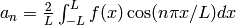 such
that
such
that
EXAMPLES:
sage: f(x) = x
sage: f = Piecewise([[(0,1),f]])
sage: f.cosine_series_coefficient(2,1)
0
sage: f.cosine_series_coefficient(3,1)
-4/9/pi^2
sage: f1(x) = -1
sage: f2(x) = 2
sage: f = Piecewise([[(0,pi/2),f1],[(pi/2,pi),f2]])
sage: f.cosine_series_coefficient(2,pi)
0
sage: f.cosine_series_coefficient(3,pi)
2/pi
sage: f.cosine_series_coefficient(111,pi)
2/37/pi
sage: f1 = lambda x: x*(pi-x)
sage: f = Piecewise([[(0,pi),f1]])
sage: f.cosine_series_coefficient(0,pi)
1/3*pi^2
Return the critical points of this piecewise function.
Warning
Uses maxima, which prints the warning to use results with caution. Only works for piecewise functions whose parts are polynomials with real critical not occurring on the interval endpoints.
EXAMPLES:
sage: R.<x> = QQ[]
sage: f1 = x^0
sage: f2 = 10*x - x^2
sage: f3 = 3*x^4 - 156*x^3 + 3036*x^2 - 26208*x
sage: f = Piecewise([[(0,3),f1],[(3,10),f2],[(10,20),f3]])
sage: expected = [5, 12, 13, 14]
sage: all(abs(e-a) < 0.001 for e,a in zip(expected, f.critical_points()))
True
Return the default variable. The default variable is defined as the
first variable in the first piece uses a variable. If no pieces have
a variable (each piece is a constant value),  is returned.
The result is cached.
AUTHOR: Paul Butler
EXAMPLES:
sage: f1(x) = 1
sage: f2(x) = 5*x
sage: p = Piecewise([[(0,1),f1],[(1,4),f2]])
sage: p.default_variable()
x

sage: f1 = 3*var('y')
sage: p = Piecewise([[(0,1),4],[(1,4),f1]])
sage: p.default_variable()
y
Returns the derivative (as computed by maxima) Piecewise(I,`(d/dx)(self|_I)`), as I runs over the intervals belonging to self. self must be piecewise polynomial.
EXAMPLES:
sage: f1(x) = 1
sage: f2(x) = 1-x
sage: f = Piecewise([[(0,1),f1],[(1,2),f2]])
sage: f.derivative()
Piecewise defined function with 2 parts, [[(0, 1), x |--> 0], [(1, 2), x |--> -1]]
sage: f1(x) = -1
sage: f2(x) = 2
sage: f = Piecewise([[(0,pi/2),f1],[(pi/2,pi),f2]])
sage: f.derivative()
Piecewise defined function with 2 parts, [[(0, 1/2*pi), x |--> 0], [(1/2*pi, pi), x |--> 0]]
sage: f = Piecewise([[(0,1), (x * 2)]], x)
sage: f.derivative()
Piecewise defined function with 1 parts, [[(0, 1), x |--> 2]]
Returns the domain of the function.
EXAMPLES:
sage: f1(x) = 1
sage: f2(x) = 1-x
sage: f3(x) = exp(x)
sage: f4(x) = sin(2*x)
sage: f = Piecewise([[(0,1),f1],[(1,2),f2],[(2,3),f3],[(3,10),f4]])
sage: f.domain()
(0, 10)
Returns a list of all interval endpoints for this function.
EXAMPLES:
sage: f1(x) = 1
sage: f2(x) = 1-x
sage: f3(x) = x^2-5
sage: f = Piecewise([[(0,1),f1],[(1,2),f2],[(2,3),f3]])
sage: f.end_points()
[0, 1, 2, 3]
This function simply returns the piecewise defined function which is extended by 0 so it is defined on all of (xmin,xmax). This is needed to add two piecewise functions in a reasonable way.
EXAMPLES:
sage: f1(x) = 1
sage: f2(x) = 1 - x
sage: f = Piecewise([[(0,1),f1],[(1,2),f2]])
sage: f.extend_by_zero_to(-1, 3)
Piecewise defined function with 4 parts, [[(-1, 0), 0], [(0, 1), x |--> 1], [(1, 2), x |--> -x + 1], [(2, 3), 0]]
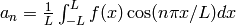
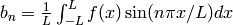
Returns the n-th Fourier series coefficient of
, .
INPUT:
OUTPUT:
EXAMPLES:
sage: f(x) = x^2
sage: f = Piecewise([[(-1,1),f]])
sage: f.fourier_series_cosine_coefficient(2,1)
pi^(-2)
sage: f(x) = x^2
sage: f = Piecewise([[(-pi,pi),f]])
sage: f.fourier_series_cosine_coefficient(2,pi)
1
sage: f1(x) = -1
sage: f2(x) = 2
sage: f = Piecewise([[(-pi,pi/2),f1],[(pi/2,pi),f2]])
sage: f.fourier_series_cosine_coefficient(5,pi)
-3/5/pi
Returns the partial sum
![f(x) \sim \frac{a_0}{2} + \sum_{n=1}^N [a_n\cos(\frac{n\pi x}{L}) + b_n\sin(\frac{n\pi x}{L})],](../../_images/math/d48564130053855c59aa81bad8da4877f87968b8.png)
as a string.
EXAMPLE:
sage: f(x) = x^2
sage: f = Piecewise([[(-1,1),f]])
sage: f.fourier_series_partial_sum(3,1)
-4*cos(pi*x)/pi^2 + cos(2*pi*x)/pi^2 + 1/3
sage: f1(x) = -1
sage: f2(x) = 2
sage: f = Piecewise([[(-pi,pi/2),f1],[(pi/2,pi),f2]])
sage: f.fourier_series_partial_sum(3,pi)
-3*sin(2*x)/pi + 3*sin(x)/pi - 3*cos(x)/pi - 1/4
Returns the Cesaro partial sum
![f(x) \sim \frac{a_0}{2} + \sum_{n=1}^N (1-n/N)*[a_n\cos(\frac{n\pi x}{L}) + b_n\sin(\frac{n\pi x}{L})],](../../_images/math/d67629b08c8a4fe87d5c0e441366794e5fc916c8.png)
as a string. This is a “smoother” partial sum - the Gibbs phenomenon is mollified.
EXAMPLE:
sage: f(x) = x^2
sage: f = Piecewise([[(-1,1),f]])
sage: f.fourier_series_partial_sum_cesaro(3,1)
-8/3*cos(pi*x)/pi^2 + 1/3*cos(2*pi*x)/pi^2 + 1/3
sage: f1(x) = -1
sage: f2(x) = 2
sage: f = Piecewise([[(-pi,pi/2),f1],[(pi/2,pi),f2]])
sage: f.fourier_series_partial_sum_cesaro(3,pi)
-sin(2*x)/pi + 2*sin(x)/pi - 2*cos(x)/pi - 1/4
Returns the “filtered” partial sum
![f(x) \sim \frac{a_0}{2} + \sum_{n=1}^N F_n*[a_n\cos(\frac{n\pi x}{L}) + b_n\sin(\frac{n\pi x}{L})],](../../_images/math/03f68cb5310cbca6e2bd0bb0d32875d2ca37ebbd.png)
as a string, where ![F = [F_1,F_2, ..., F_{N}]](../../_images/math/b4e3544e2ae30045c33abc556c05ff4ee5d04eb1.png) is a list
of length
is a list
of length  consisting of real numbers. This can be used
to plot FS solutions to the heat and wave PDEs.
consisting of real numbers. This can be used
to plot FS solutions to the heat and wave PDEs.
EXAMPLE:
sage: f(x) = x^2
sage: f = Piecewise([[(-1,1),f]])
sage: f.fourier_series_partial_sum_filtered(3,1,[1,1,1])
-4*cos(pi*x)/pi^2 + cos(2*pi*x)/pi^2 + 1/3
sage: f1(x) = -1
sage: f2(x) = 2
sage: f = Piecewise([[(-pi,pi/2),f1],[(pi/2,pi),f2]])
sage: f.fourier_series_partial_sum_filtered(3,pi,[1,1,1])
-3*sin(2*x)/pi + 3*sin(x)/pi - 3*cos(x)/pi - 1/4
Returns the Hann-filtered partial sum (named after von Hann, not Hamming)
![f(x) \sim \frac{a_0}{2} + \sum_{n=1}^N H_N(n)*[a_n\cos(\frac{n\pi x}{L}) + b_n\sin(\frac{n\pi x}{L})],](../../_images/math/984470ae99e20cc112bc72637088b15ce6fb7543.png)
as a string, where  . This is
a “smoother” partial sum - the Gibbs phenomenon is mollified.
. This is
a “smoother” partial sum - the Gibbs phenomenon is mollified.
EXAMPLE:
sage: f(x) = x^2
sage: f = Piecewise([[(-1,1),f]])
sage: f.fourier_series_partial_sum_hann(3,1)
-3*cos(pi*x)/pi^2 + 1/4*cos(2*pi*x)/pi^2 + 1/3
sage: f1(x) = -1
sage: f2(x) = 2
sage: f = Piecewise([[(-pi,pi/2),f1],[(pi/2,pi),f2]])
sage: f.fourier_series_partial_sum_hann(3,pi)
-3/4*sin(2*x)/pi + 9/4*sin(x)/pi - 9/4*cos(x)/pi - 1/4
Returns the n-th Fourier series coefficient of
 ,
,  .
.
INPUT:
OUTPUT:
EXAMPLES:
sage: f(x) = x^2
sage: f = Piecewise([[(-1,1),f]])
sage: f.fourier_series_sine_coefficient(2,1)  # L=1, n=2
0
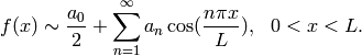
Returns the value of the Fourier series coefficient of self at
,
![f(x) \sim \frac{a_0}{2} + \sum_{n=1}^\infty [a_n\cos(\frac{n\pi x}{L}) + b_n\sin(\frac{n\pi x}{L})], \ \ \ -L<x<L.](../../_images/math/6b48d87fe381c7cdba200bb5e6e4993b3ee389a6.png)
This method applies to piecewise non-polynomial functions as well.
INPUT:
OUTPUT:  , where
  denotes
the function
denotes
the function  extended to
  with period
 (Dirichlet’s Theorem for Fourier series).
EXAMPLES:
sage: f1(x) = 1
sage: f2(x) = 1-x
sage: f3(x) = exp(x)
sage: f4(x) = sin(2*x)
sage: f = Piecewise([[(-10,1),f1],[(1,2),f2],[(2,3),f3],[(3,10),f4]])
sage: f.fourier_series_value(101,10)
1/2
sage: f.fourier_series_value(100,10)
1
sage: f.fourier_series_value(10,10)
1/2*sin(20) + 1/2
sage: f.fourier_series_value(20,10)
1
sage: f.fourier_series_value(30,10)
1/2*sin(20) + 1/2
sage: f1(x) = -1
sage: f2(x) = 2
sage: f = Piecewise([[(-pi,0),lambda x:0],[(0,pi/2),f1],[(pi/2,pi),f2]])
sage: f.fourier_series_value(-1,pi)
0
sage: f.fourier_series_value(20,pi)
-1
sage: f.fourier_series_value(pi/2,pi)
1/2
Returns the list of functions (the “pieces”).
EXAMPLES:
sage: f1(x) = 1
sage: f2(x) = 1-x
sage: f3(x) = exp(x)
sage: f4(x) = sin(2*x)
sage: f = Piecewise([[(0,1),f1],[(1,2),f2],[(2,3),f3],[(3,10),f4]])
sage: f.functions()
[x |--> 1, x |--> -x + 1, x |--> e^x, x |--> sin(2*x)]
By default, returns the indefinite integral of the function. If definite=True is given, returns the definite integral.
AUTHOR:
EXAMPLES:
sage: f1(x) = 1-x
sage: f = Piecewise([[(0,1),1],[(1,2),f1]])
sage: f.integral(definite=True)
1/2
sage: f1(x) = -1
sage: f2(x) = 2
sage: f = Piecewise([[(0,pi/2),f1],[(pi/2,pi),f2]])
sage: f.integral(definite=True)
1/2*pi

sage: f1(x) = 2
sage: f2(x) = 3 - x
sage: f = Piecewise([[(-2, 0), f1], [(0, 3), f2]])
sage: f.integral()
Piecewise defined function with 2 parts, [[(-2, 0), x |--> 2*x + 4], [(0, 3), x |--> -1/2*x^2 + 3*x + 4]]

sage: f1(y) = -1
sage: f2(y) = y + 3
sage: f3(y) = -y - 1
sage: f4(y) = y^2 - 1
sage: f5(y) = 3
sage: f = Piecewise([[(-4,-3),f1],[(-3,-2),f2],[(-2,0),f3],[(0,2),f4],[(2,3),f5]])
sage: F = f.integral(y)
sage: F
Piecewise defined function with 5 parts, [[(-4, -3), y |--> -y - 4], [(-3, -2), y |--> 1/2*y^2 + 3*y + 7/2], [(-2, 0), y |--> -1/2*y^2 - y - 1/2], [(0, 2), y |--> 1/3*y^3 - y - 1/2], [(2, 3), y |--> 3*y - 35/6]]
Ensure results are consistent with FTC:
sage: F(-3) - F(-4)
-1
sage: F(-1) - F(-3)
1
sage: F(2) - F(0)
2/3
sage: f.integral(y, 0, 2)
2/3
sage: F(3) - F(-4)
19/6
sage: f.integral(y, -4, 3)
19/6
sage: f.integral(definite=True)
19/6
sage: f1(y) = (y+3)^2
sage: f2(y) = y+3
sage: f3(y) = 3
sage: f = Piecewise([[(-infinity, -3), f1], [(-3, 0), f2], [(0, infinity), f3]])
sage: f.integral()
Piecewise defined function with 3 parts, [[(-Infinity, -3), y |--> 1/3*y^3 + 3*y^2 + 9*y + 9], [(-3, 0), y |--> 1/2*y^2 + 3*y + 9/2], [(0, +Infinity), y |--> 3*y + 9/2]]
sage: f1(x) = e^(-abs(x))
sage: f = Piecewise([[(-infinity, infinity), f1]])
sage: f.integral(definite=True)
2
sage: f.integral()
Piecewise defined function with 1 parts, [[(-Infinity, +Infinity), x |--> -integrate(e^(-abs(x)), x, x, +Infinity)]]
sage: f = Piecewise([((0, 5), cos(x))])
sage: f.integral()
Piecewise defined function with 1 parts, [[(0, 5), x |--> sin(x)]]
A piecewise non-polynomial example.
EXAMPLES:
sage: f1(x) = 1
sage: f2(x) = 1-x
sage: f3(x) = exp(x)
sage: f4(x) = sin(2*x)
sage: f = Piecewise([[(0,1),f1],[(1,2),f2],[(2,3),f3],[(3,10),f4]])
sage: f.intervals()
[(0, 1), (1, 2), (2, 3), (3, 10)]
Returns the Laplace transform of self with respect to the variable var.
INPUT:
We assume that a piecewise function is 0 outside of its domain and that the left-most endpoint of the domain is 0.
EXAMPLES:
sage: x, s, w = var('x, s, w')
sage: f = Piecewise([[(0,1),1],[(1,2), 1-x]])
sage: f.laplace(x, s)
(s + 1)*e^(-2*s)/s^2 - e^(-s)/s + 1/s - e^(-s)/s^2
sage: f.laplace(x, w)
(w + 1)*e^(-2*w)/w^2 - e^(-w)/w + 1/w - e^(-w)/w^2
sage: y, t = var('y, t')
sage: f = Piecewise([[(1,2), 1-y]])
sage: f.laplace(y, t)
(t + 1)*e^(-2*t)/t^2 - e^(-t)/t^2
sage: s = var('s')
sage: t = var('t')
sage: f1(t) = -t
sage: f2(t) = 2
sage: f = Piecewise([[(0,1),f1],[(1,infinity),f2]])
sage: f.laplace(t,s)
(s + 1)*e^(-s)/s^2 + 2*e^(-s)/s - 1/s^2
Returns the number of pieces of this function.
EXAMPLES:
sage: f1(x) = 1
sage: f2(x) = 1 - x
sage: f = Piecewise([[(0,1),f1],[(1,2),f2]])
sage: f.length()
2
Returns the pieces of this function as a list of functions.
EXAMPLES:
sage: f1(x) = 1
sage: f2(x) = 1 - x
sage: f = Piecewise([[(0,1),f1],[(1,2),f2]])
sage: f.list()
[[(0, 1), x |--> 1], [(1, 2), x |--> -x + 1]]
Returns the plot of self.
Keyword arguments are passed onto the plot command for each piece of the function. E.g., the plot_points keyword affects each segment of the plot.
EXAMPLES:
sage: f1(x) = 1
sage: f2(x) = 1-x
sage: f3(x) = exp(x)
sage: f4(x) = sin(2*x)
sage: f = Piecewise([[(0,1),f1],[(1,2),f2],[(2,3),f3],[(3,10),f4]])
sage: P = f.plot(rgbcolor=(0.7,0.1,0), plot_points=40)
sage: P
Remember: to view this, type show(P) or P.save(“path/myplot.png”) and then open it in a graphics viewer such as GIMP.
Plots the partial sum
![f(x) \sim \frac{a_0}{2} + sum_{n=1}^N [a_n\cos(\frac{n\pi x}{L}) + b_n\sin(\frac{n\pi x}{L})],](../../_images/math/3c129f4c682423e15749259a7ad61159fe89a0f7.png)
over xmin x xmin.
EXAMPLE:
sage: f1(x) = -2
sage: f2(x) = 1
sage: f3(x) = -1
sage: f4(x) = 2
sage: f = Piecewise([[(-pi,-pi/2),f1],[(-pi/2,0),f2],[(0,pi/2),f3],[(pi/2,pi),f4]])
sage: P = f.plot_fourier_series_partial_sum(3,pi,-5,5)    # long time
sage: f1(x) = -1
sage: f2(x) = 2
sage: f = Piecewise([[(-pi,pi/2),f1],[(pi/2,pi),f2]])
sage: P = f.plot_fourier_series_partial_sum(15,pi,-5,5)   # long time
Remember, to view this type show(P) or P.save(“path/myplot.png”) and then open it in a graphics viewer such as GIMP.
Plots the partial sum
![f(x) \sim \frac{a_0}{2} + \sum_{n=1}^N (1-n/N)*[a_n\cos(\frac{n\pi x}{L}) + b_n\sin(\frac{n\pi x}{L})],](../../_images/math/ae5d9ffb5dad30346a786fb9bc2fb9fefb96190e.png)
over xmin x xmin. This is a “smoother” partial sum - the Gibbs phenomenon is mollified.
EXAMPLE:
sage: f1(x) = -2
sage: f2(x) = 1
sage: f3(x) = -1
sage: f4(x) = 2
sage: f = Piecewise([[(-pi,-pi/2),f1],[(-pi/2,0),f2],[(0,pi/2),f3],[(pi/2,pi),f4]])
sage: P = f.plot_fourier_series_partial_sum_cesaro(3,pi,-5,5)    # long time
sage: f1(x) = -1
sage: f2(x) = 2
sage: f = Piecewise([[(-pi,pi/2),f1],[(pi/2,pi),f2]])
sage: P = f.plot_fourier_series_partial_sum_cesaro(15,pi,-5,5)   # long time
Remember, to view this type show(P) or P.save(“path/myplot.png”) and then open it in a graphics viewer such as GIMP.
Plots the partial sum
![f(x) \sim \frac{a_0}{2} + \sum_{n=1}^N F_n*[a_n\cos(\frac{n\pi x}{L}) + b_n\sin(\frac{n\pi x}{L})],](../../_images/math/9d47d8b6349431a3d71aa45ffcd9df0750be0584.png)
over xmin x xmin, where is a
list of length consisting of real numbers. This can be
used to plot FS solutions to the heat and wave PDEs.
EXAMPLE:
sage: f1(x) = -2
sage: f2(x) = 1
sage: f3(x) = -1
sage: f4(x) = 2
sage: f = Piecewise([[(-pi,-pi/2),f1],[(-pi/2,0),f2],[(0,pi/2),f3],[(pi/2,pi),f4]])
sage: P = f.plot_fourier_series_partial_sum_filtered(3,pi,[1]*3,-5,5)    # long time
sage: f1(x) = -1
sage: f2(x) = 2
sage: f = Piecewise([[(-pi,-pi/2),f1],[(-pi/2,0),f2],[(0,pi/2),f1],[(pi/2,pi),f2]])
sage: P = f.plot_fourier_series_partial_sum_filtered(15,pi,[1]*15,-5,5)   # long time
Remember, to view this type show(P) or P.save(“path/myplot.png”) and then open it in a graphics viewer such as GIMP.
Plots the partial sum
over xmin x xmin, where H_N(x) = (0.5)+(0.5)*cos(x*pi/N) is the N-th Hann filter.
EXAMPLE:
sage: f1(x) = -2
sage: f2(x) = 1
sage: f3(x) = -1
sage: f4(x) = 2
sage: f = Piecewise([[(-pi,-pi/2),f1],[(-pi/2,0),f2],[(0,pi/2),f3],[(pi/2,pi),f4]])
sage: P = f.plot_fourier_series_partial_sum_hann(3,pi,-5,5)    # long time
sage: f1(x) = -1
sage: f2(x) = 2
sage: f = Piecewise([[(-pi,pi/2),f1],[(pi/2,pi),f2]])
sage: P = f.plot_fourier_series_partial_sum_hann(15,pi,-5,5)   # long time
Remember, to view this type show(P) or P.save(“path/myplot.png”) and then open it in a graphics viewer such as GIMP.
Returns the piecewise line function defined by the Riemann sums in numerical integration based on a subdivision into N subintervals. Set mode=”midpoint” for the height of the rectangles to be determined by the midpoint of the subinterval; set mode=”right” for the height of the rectangles to be determined by the right-hand endpoint of the subinterval; the default is mode=”left” (the height of the rectangles to be determined by the left-hand endpoint of the subinterval).
EXAMPLES:
sage: f1(x) = x^2
sage: f2(x) = 5-x^2
sage: f = Piecewise([[(0,1),f1],[(1,2),f2]])
sage: f.riemann_sum(6,mode="midpoint")
Piecewise defined function with 6 parts, [[(0, 1/3), 1/36], [(1/3, 2/3), 1/4], [(2/3, 1), 25/36], [(1, 4/3), 131/36], [(4/3, 5/3), 11/4], [(5/3, 2), 59/36]]
sage: f = Piecewise([[(-1,1),(1-x^2).function(x)]])
sage: rsf = f.riemann_sum(7)
sage: P = f.plot(rgbcolor=(0.7,0.1,0.5), plot_points=40)
sage: Q = rsf.plot(rgbcolor=(0.7,0.6,0.6), plot_points=40)
sage: L = add([line([[a,0],[a,f(x=a)]],rgbcolor=(0.7,0.6,0.6)) for (a,b),f in rsf.list()])
sage: P + Q + L
sage: f = Piecewise([[(-1,1),(1/2+x-x^3)]], x) ## example 3
sage: rsf = f.riemann_sum(8)
sage: P = f.plot(rgbcolor=(0.7,0.1,0.5), plot_points=40)
sage: Q = rsf.plot(rgbcolor=(0.7,0.6,0.6), plot_points=40)
sage: L = add([line([[a,0],[a,f(x=a)]],rgbcolor=(0.7,0.6,0.6)) for (a,b),f in rsf.list()])
sage: P + Q + L
Returns the piecewise line function defined by the Riemann sums in numerical integration based on a subdivision into N subintervals.
Set mode=”midpoint” for the height of the rectangles to be determined by the midpoint of the subinterval; set mode=”right” for the height of the rectangles to be determined by the right-hand endpoint of the subinterval; the default is mode=”left” (the height of the rectangles to be determined by the left-hand endpoint of the subinterval).
EXAMPLES:
sage: f1(x) = x^2                   ## example 1
sage: f2(x) = 5-x^2
sage: f = Piecewise([[(0,1),f1],[(1,2),f2]])
sage: f.riemann_sum_integral_approximation(6)
17/6
sage: f.riemann_sum_integral_approximation(6,mode="right")
19/6
sage: f.riemann_sum_integral_approximation(6,mode="midpoint")
3
sage: f.integral(definite=True)
3
Returns the n-th sine series coefficient of
, .
INPUT:
OUTPUT:
 such
that
such
that
EXAMPLES:
sage: f(x) = 1
sage: f = Piecewise([[(0,1),f]])
sage: f.sine_series_coefficient(2,1)
0
sage: f.sine_series_coefficient(3,1)
4/3/pi
Computes the linear function defining the tangent line of the piecewise function self.
EXAMPLES:
sage: f1(x) = x^2
sage: f2(x) = 5-x^3+x
sage: f = Piecewise([[(0,1),f1],[(1,2),f2]])
sage: tf = f.tangent_line(0.9) ## tangent line at x=0.9
sage: P = f.plot(rgbcolor=(0.7,0.1,0.5), plot_points=40)
sage: Q = tf.plot(rgbcolor=(0.7,0.2,0.2), plot_points=40)
sage: P + Q
Returns the piecewise line function defined by the trapezoid rule for numerical integration based on a subdivision into N subintervals.
EXAMPLES:
sage: R.<x> = QQ[]
sage: f1 = x^2
sage: f2 = 5-x^2
sage: f = Piecewise([[(0,1),f1],[(1,2),f2]])
sage: f.trapezoid(4)
Piecewise defined function with 4 parts, [[(0, 1/2), 1/2*x], [(1/2, 1), 9/2*x - 2], [(1, 3/2), 1/2*x + 2], [(3/2, 2), -7/2*x + 8]]
sage: R.<x> = QQ[]
sage: f = Piecewise([[(-1,1),1-x^2]])
sage: tf = f.trapezoid(4)
sage: P = f.plot(rgbcolor=(0.7,0.1,0.5), plot_points=40)
sage: Q = tf.plot(rgbcolor=(0.7,0.6,0.6), plot_points=40)
sage: L = add([line([[a,0],[a,f(a)]],rgbcolor=(0.7,0.6,0.6)) for (a,b),f in tf.list()])
sage: P+Q+L
sage: R.<x> = QQ[]
sage: f = Piecewise([[(-1,1),1/2+x-x^3]]) ## example 3
sage: tf = f.trapezoid(6)
sage: P = f.plot(rgbcolor=(0.7,0.1,0.5), plot_points=40)
sage: Q = tf.plot(rgbcolor=(0.7,0.6,0.6), plot_points=40)
sage: L = add([line([[a,0],[a,f(a)]],rgbcolor=(0.7,0.6,0.6)) for (a,b),f in tf.list()])
sage: P+Q+L
Returns the approximation given by the trapezoid rule for numerical integration based on a subdivision into N subintervals.
EXAMPLES:
sage: f1(x) = x^2                      ## example 1
sage: f2(x) = 1-(1-x)^2
sage: f = Piecewise([[(0,1),f1],[(1,2),f2]])
sage: P = f.plot(rgbcolor=(0.7,0.1,0.5), plot_points=40)
sage: tf = f.trapezoid(6)
sage: Q = tf.plot(rgbcolor=(0.7,0.6,0.6), plot_points=40)
sage: ta = f.trapezoid_integral_approximation(6)
sage: t = text('trapezoid approximation = %s'%ta, (1.5, 0.25))
sage: a = f.integral(definite=True)
sage: tt = text('area under curve = %s'%a, (1.5, -0.5))
sage: P + Q + t + tt
sage: f = Piecewise([[(0,1),f1],[(1,2),f2]])  ## example 2
sage: tf = f.trapezoid(4)
sage: ta = f.trapezoid_integral_approximation(4)
sage: Q = tf.plot(rgbcolor=(0.7,0.6,0.6), plot_points=40)
sage: t = text('trapezoid approximation = %s'%ta, (1.5, 0.25))
sage: a = f.integral(definite=True)
sage: tt = text('area under curve = %s'%a, (1.5, -0.5))
sage: P+Q+t+tt
This removes any parts in the front or back of the function which is zero (the inverse to extend_by_zero_to).
EXAMPLES:
sage: R.<x> = QQ[]
sage: f = Piecewise([[(-3,-1),1+2+x],[(-1,1),1-x^2]])
sage: e = f.extend_by_zero_to(-10,10); e
Piecewise defined function with 4 parts, [[(-10, -3), 0], [(-3, -1), x + 3], [(-1, 1), -x^2 + 1], [(1, 10), 0]]
sage: d = e.unextend(); d
Piecewise defined function with 2 parts, [[(-3, -1), x + 3], [(-1, 1), -x^2 + 1]]
sage: d==f
True
Returns the function piece used to evaluate self at x0.
EXAMPLES:
sage: f1(z) = z
sage: f2(x) = 1-x
sage: f3(y) = exp(y)
sage: f4(t) = sin(2*t)
sage: f = Piecewise([[(0,1),f1],[(1,2),f2],[(2,3),f3],[(3,10),f4]])
sage: f.which_function(3/2)
x |--> -x + 1
Returns a piecewise function from a list of (interval, function) pairs.
list_of_pairs is a list of pairs (I, fcn), where fcn is a Sage function (such as a polynomial over RR, or functions using the lambda notation), and I is an interval such as I = (1,3). Two consecutive intervals must share a common endpoint.
If the optional var is specified, then any symbolic expressions in the list will be converted to symbolic functions using fcn.function(var). (This says which variable is considered to be “piecewise”.)
We assume that these definitions are consistent (ie, no checking is done).
EXAMPLES:
sage: f1(x) = -1
sage: f2(x) = 2
sage: f = Piecewise([[(0,pi/2),f1],[(pi/2,pi),f2]])
sage: f(1)
-1
sage: f(3)
2
sage: f = Piecewise([[(0,1),x], [(1,2),x^2]], x); f
Piecewise defined function with 2 parts, [[(0, 1), x |--> x], [(1, 2), x |--> x^2]]
sage: f(0.9)
0.900000000000000
sage: f(1.1)
1.21000000000000
