Transcendental Functions¶

class sage.functions.transcendental.DickmanRho¶

Bases: sage.symbolic.function.BuiltinFunction

Dickman’s function is the continuous function satisfying the differential equation

$x \rho'(x) + \rho(x-1) = 0$

with initial conditions $\rho(x)=1$ for $0 \le x \le 1$ . It is useful in estimating the frequency of smooth numbers as asymptotically

$\Psi(a, a^{1/s}) \sim a \rho(s)$

where $\Psi(a,b)$ is the number of $b$ -smooth numbers less than $a$ .

ALGORITHM:

Dickmans’s function is analytic on the interval $[n,n+1]$ for each integer $n$ . To evaluate at $n+t, 0 \le t < 1$ , a power series is recursively computed about $n+1/2$ using the differential equation stated above. As high precision arithmetic may be needed for intermediate results the computed series are cached for later use.

Simple explicit formulas are used for the intervals [0,1] and [1,2].

EXAMPLES:

sage: dickman_rho(2)
0.306852819440055
sage: dickman_rho(10)
2.77017183772596e-11
sage: dickman_rho(10.00000000000000000000000000000000000000)
2.77017183772595898875812120063434232634e-11
sage: plot(log(dickman_rho(x)), (x, 0, 15))

AUTHORS:

Robert Bradshaw (2008-09)

REFERENCES:

G. Marsaglia, A. Zaman, J. Marsaglia. “Numerical Solutions to some Classical Differential-Difference Equations.” Mathematics of Computation, Vol. 53, No. 187 (1989).

approximate(x, parent=None)¶

Approximate using de Bruijn’s formula

$\rho(x) \sim \frac{exp(-x \xi + Ei(\xi))}{\sqrt{2\pi x}\xi}$

which is asymptotically equal to Dickman’s function, and is much faster to compute.

REFERENCES:

N. De Bruijn, “The Asymptotic behavior of a function occurring in the theory of primes.” J. Indian Math Soc. v 15. (1951)

EXAMPLES:

sage: dickman_rho.approximate(10)
2.41739196365564e-11
sage: dickman_rho(10)
2.77017183772596e-11
sage: dickman_rho.approximate(1000)
4.32938809066403e-3464

power_series(n, abs_prec)¶

This function returns the power series about $n+1/2$ used to evaluate Dickman’s function. It is scaled such that the interval $[n,n+1]$ corresponds to x in $[-1,1]$ .

INPUT:

n - the lower endpoint of the interval for which this power series holds
abs_prec - the absolute precision of the resulting power series

EXAMPLES:

sage: f = dickman_rho.power_series(2, 20); f
-9.9376e-8*x^11 + 3.7722e-7*x^10 - 1.4684e-6*x^9 + 5.8783e-6*x^8 - 0.000024259*x^7 + 0.00010341*x^6 - 0.00045583*x^5 + 0.0020773*x^4 - 0.0097336*x^3 + 0.045224*x^2 - 0.11891*x + 0.13032
sage: f(-1), f(0), f(1)
(0.30685, 0.13032, 0.048608)
sage: dickman_rho(2), dickman_rho(2.5), dickman_rho(3)
(0.306852819440055, 0.130319561832251, 0.0486083882911316)

class sage.functions.transcendental.Function_exp_integral¶: Bases: sage.symbolic.function.BuiltinFunction

class sage.functions.transcendental.Function_zeta¶: Bases: sage.symbolic.function.GinacFunction

class sage.functions.transcendental.Function_zetaderiv¶: Bases: sage.symbolic.function.GinacFunction

sage.functions.transcendental.Li(x, eps_rel=None, err_bound=False)¶

Return value of the function Li(x) as a real double field element.

This is the function

$\int_2^{x} dt / \log(t).$

The function Li(x) is an approximation for the number of primes up to $x$ . In fact, the famous Riemann Hypothesis is equivalent to the statement that for $x \geq 2.01$ we have

$|\pi(x) - Li(x)| \leq \sqrt{x} \log(x).$

For “small” $x$ , $Li(x)$ is always slightly bigger than $\pi(x)$ . However it is a theorem that there are (very large, e.g., around $10^{316}$ ) values of $x$ so that $\pi(x) > Li(x)$ . See “A new bound for the smallest x with $\pi(x) > li(x)$ “, Bays and Hudson, Mathematics of Computation, 69 (2000) 1285-1296.

ALGORITHM: Computed numerically using GSL.

INPUT:

x - a real number = 2.

OUTPUT:

x - a real double

EXAMPLES:

sage: Li(2)
0.0
sage: Li(5)
2.58942452992
sage: Li(1000)
176.56449421
sage: Li(10^5)
9628.76383727
sage: prime_pi(10^5)
9592
sage: Li(1)
...
ValueError: Li only defined for x at least 2.    

sage: for n in range(1,7):
...    print '%-10s%-10s%-20s'%(10^n, prime_pi(10^n), Li(10^n))
10        4         5.12043572467       
100       25        29.080977804        
1000      168       176.56449421        
10000     1229      1245.09205212       
100000    9592      9628.76383727       
1000000   78498     78626.5039957

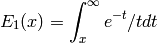
sage.functions.transcendental.exponential_integral_1(x, n=0)¶

Returns the exponential integral $E_1(x)$ . If the optional argument $n$ is given, computes list of the first $n$ values of the exponential integral $E_1(x m)$ .

The exponential integral $E_1(x)$ is

$E_1(x) = \int_{x}^{\infty} e^{-t}/t dt$

INPUT:

x - a positive real number
n - (default: 0) a nonnegative integer; if nonzero, then return a list of values E_1(x*m) for m = 1,2,3,...,n. This is useful, e.g., when computing derivatives of L-functions.

OUTPUT:

float - if n is 0 (the default) or
list - list of floats if n 0

EXAMPLES:

sage: exponential_integral_1(2)
0.048900510708061118
sage: w = exponential_integral_1(2,4); w
[0.048900510708061118, 0.0037793524098489067, 0.00036008245216265873, 3.7665622843924751e-05] # 32-bit
[0.048900510708061118, 0.0037793524098489063, 0.00036008245216265873, 3.7665622843924534e-05] # 64-bit

IMPLEMENTATION: We use the PARI C-library functions eint1 and veceint1.

REFERENCE:

See page 262, Prop 5.6.12, of Cohen’s book “A Course in Computational Algebraic Number Theory”.

REMARKS: When called with the optional argument n, the PARI C-library is fast for values of n up to some bound, then very very slow. For example, if x=5, then the computation takes less than a second for n=800000, and takes “forever” for n=900000.

sage.functions.transcendental.zeta_symmetric(s)¶

Completed function $\xi(s)$ that satisfies $\xi(s) = \xi(1-s)$ and has zeros at the same points as the Riemann zeta function.

INPUT:

s - real or complex number

If s is a real number the computation is done using the MPFR library. When the input is not real, the computation is done using the PARI C library.

More precisely,

$xi(s) = \gamma(s/2 + 1) * (s-1) * \pi^{-s/2} * \zeta(s).$

EXAMPLES:

sage: zeta_symmetric(0.7)
0.497580414651127
sage: zeta_symmetric(1-0.7)
0.497580414651127
sage: RR = RealField(200)
sage: zeta_symmetric(RR(0.7))
0.49758041465112690357779107525638385212657443284080589766062
sage: C.<i> = ComplexField()
sage: zeta_symmetric(0.5 + i*14.0)
0.000201294444235258 + 1.49077798716757e-19*I
sage: zeta_symmetric(0.5 + i*14.1)
0.0000489893483255687 + 4.40457132572236e-20*I
sage: zeta_symmetric(0.5 + i*14.2)
-0.0000868931282620101 + 7.11507675693612e-20*I

REFERENCE:

I copied the definition of xi from http://www.math.ubc.ca/~pugh/RiemannZeta/RiemannZetaLong.html

Transcendental Functions¶

Previous topic

Next topic

This Page

Navigation

Transcendental Functions¶

Previous topic

Next topic

This Page

Quick search

Navigation