Linear Programming¶

Basics¶

What is a linear program?¶

A linear program consists of the following two pieces of information:

A linear function, called the objective function, which is to be maximized or minimized, e.g. $2 x + y$ .
Linear constraints on the variables, e.g. $3 x + y \leq 2$ and $2 x + 3 y \leq 8$ .

A linear program solver would then try to find a solution to the system of constraints such that the objective function is optimized, and return specific values for the variables.

What is a mixed integer linear program?¶

A mixed integer linear program is a linear program such that some variables are forced to take integer values instead of real values. This difference affects the time required to solve a particular linear program. Indeed, solving a linear program can be done in polynomial time while solving a general mixed integer linear program is usually $NP$ -complete, i.e. it can take exponential time, according to a widely-held belief that $P \neq NP$ .

Why is linear programming so useful?¶

Linear programming is very useful in many optimization and graph-theoretic problems because of its wide range of expression. A linear program can be written to solve a problem whose solution could be obtained within reasonable time using the wealth of heuristics already contained in linear program solvers. It is often difficult to theoretically determine the execution time of a linear program, though it could produce very interesting results in practice.

For more information, consult the Wikipedia page dedicated to linear programming: http://en.wikipedia.org/wiki/Linear_programming

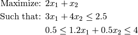
How can I solve a linear program using Sage?¶

Sage can solve linear programs or mixed integer linear programs through the class MixedIntegerLinearProgram defined in sage.numerical.mip. To illustrate how it can be used, we will try to solve the following problem:

$\text{Maximize: } & 2 x_1 + x_2 \\ \text{Such that: } & 3 x_1 + 4 x_2 \leq 2.5 \\ & 0.5 \leq 1.2 x_1 + 0.5 x_2 \leq 4$

First, we need to discuss MIPVariable and how to read the optimal values when the solver has finished its job.

Variables in `MixedIntegerLinearProgram`¶

A variable linked to an instance of MixedIntegerLinearProgram behaves exactly as a dictionary would. It is declared as follows:

sage: p = MixedIntegerLinearProgram()
sage: variable = p.new_variable()

The variable variable can contain as many keys as you like, where each key must be unique. For example, the following constraint (where $P$ denotes pressure and $T$ temperature)

$2 T_{\text{Madrid}} + 3 T_{\text{London}} - P_{\text{Seattle}} + \text{flow}_{3, 5} + 8 \text{cost}_{(1, 3)} + x_3 < 5$

can be written as:

sage: p = MixedIntegerLinearProgram()
sage: temperature = p.new_variable()
sage: pressure = p.new_variable()
sage: x = p.new_variable()
sage: cost = p.new_variable()
sage: flow = p.new_variable(dim=2)
sage: p.add_constraint(2*temperature["Madrid"] + 3*temperature["London"] - pressure["Seattle"] + flow[3][5] + 8*cost[(1, 3)] + x[3], max=5)

This example shows different possibilities for using the MixedIntegerLinearProgram class. You would not need to declare so many variables in some common applications of linear programming.

Notice how the variable flow is defined: you can use any hashable object as a key for a MIPVariable, but if you think you need more than one dimension, you need to explicitly specify it when calling MixedIntegerLinearProgram.new_variable().

For the user’s convenience, there is a default variable attached to a linear program. The above code listing means that each variable actually represents a property of a set of objects (these objects are strings in the case of temperature or a pair in the case of cost). In some cases, it is useful to define an absolute variable which will not be indexed on anything. This can be done as follows:

sage: p = MixedIntegerLinearProgram()
sage: B = p.new_variable()
sage: p.set_objective(p["first unique variable"] + B[2] + p[-3])

In this case, two of these “unique” variables are defined through p["first unique variable"] and p[-3].

Let’s solve this system¶

Now that we know what variables are, we are only several steps away from solving our system:

sage: # First, we define our MixedIntegerLinearProgram object,
sage: # setting maximization=True.
sage: p = MixedIntegerLinearProgram(maximization=True)
sage: x = p.new_variable()
sage: # Definition of the objective function
sage: p.set_objective(2*x[1] + x[2])
sage: # Next, the two constraints
sage: p.add_constraint(3*x[1] + 4*x[2], max=2.5)
sage: p.add_constraint(1.5*x[1]+0.5*x[2], max=4, min=0.5)
sage: p.solve()                # optional - requires GLPK or COIN-OR/CBC
1.6666666666666667
sage: x_sol = p.get_values(x)  # optional - requires GLPK or COIN-OR/CBC
sage: print x_sol              # optional - requires GLPK or COIN-OR/CBC
{1: 0.83333333333333337, 2: 0.0}

The value returned by MixedIntegerLinearProgram.solve() is the optimal value of the objective function. To read the values taken by the variables, one needs to call the method MixedIntegerLinearProgram.get_values() which can return multiple values at the same time if needed (type MixedIntegerLinearProgram.get_values? for more information on this function).

Some famous examples¶

Vertex cover in a graph¶

Let $G = (V, E)$ be a graph with vertex set $V$ and edge set $E$ . In the vertex cover problem, we are given $G$ and we want to find a subset $S \subseteq V$ of minimal cardinality such that each edge $e$ is incident to at least one vertex in $S$ . In order to achieve this, we define a binary variable $b_v$ for each vertex $v$ . The vertex cover problem can be expressed as the following linear program:

$\text{Maximize: } & \sum_{v \in V} b_v \\ \text{Such that: } & \forall (u, v) \in E, b_u + b_v \geq 1 \\ & \forall v, b_v \text{ is a binary variable}$

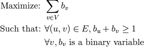
In the linear program, the syntax is exactly the same:

sage: g = graphs.PetersenGraph()
sage: p = MixedIntegerLinearProgram(maximization=False)
sage: b = p.new_variable()
sage: for u, v in g.edges(labels=None):
...       p.add_constraint(b[u] + b[v], min=1)
sage: p.set_binary(b)

And you need to type p.solve() to see the result.

Maximum matching in a graph¶

In the maximum matching problem, we are given a graph $G = (V, E)$ and we want a set of edges $M \subseteq E$ of maximum cardinality such that no two edges from $M$ are adjacent:

$\text{Maximize: } & \sum_{e \in E} b_e \\ \text{Such that: } & \forall v \in V, \sum_{(v,u) \in E} b_{vu} \leq 1 \\ & \forall e \in E, b_e \text{ is a binary variable}$

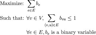
Here, we use Sage to solve the maximum matching problem for the case of the Petersen graph:

sage: g = graphs.PetersenGraph()
sage: p = MixedIntegerLinearProgram()
sage: b = p.new_variable(dim=2)
sage: for u in g.vertices():
...       p.add_constraint(sum([b[u][v] for v in g.neighbors(u)]), max=1)
sage: for u, v in g.edges(labels=None):
...       p.add_constraint(b[u][v] + b[v][u], min=1, max=1)

And the next step is p.solve().

Solvers¶

Sage solves linear programs by calling specific libraries. The following libraries are currently supported :

CBC: A solver from from COIN-OR (CPL – Free)
CPLEX: A solver from ILOG (Proprietary)
GLPK: A solver from GNU (GPL3, Free)

Installing GLPK or CBC¶

GPLK and CBC being free softwares, they can be easily installed as follows:

sage: # To install GLPK
sage: install_package("glpk")  # not tested
sage: # To install COIN-OR Branch and Cut (CBC)
sage: install_package("cbc")   # not tested

Installing CPLEX¶

ILOG CPLEX, on the other hand, is Proprietary – to use it through Sage, you must first be in possession of :

A valid license file
A compiled version of the CPLEX library (usually named libcplex.a)
The header file cplex.h

The license file path must be set the value of the environment variable ILOG_LICENSE_FILE. For example, you can write

export ILOG_LICENSE_FILE=/path/to/the/license/ilog/ilm/access_1.ilm

at the end of your .bashrc file.

As Sage also needs the files libcplex.a and cplex.h, the easiest way is to create symbolic links toward these files in the appropriate directories :

libcplex.a – in SAGE_ROOT/local/lib/, type
```
ln -s /path/to/lib/libcplex.a .
```
cplex.h – in SAGE_ROOT/local/include/, type
```
ln -s /path/to/include/cplex.h .
```

Once this is done, and as CPLEX is used in Sage through the Osi library, which is part of the Cbc package, you can type:

sage: install_package("cbc")  # not tested

or, if you had already installed Cbc

sage: install_package("cbc", force = True)  # not tested

to reinstall it.

Linear Programming¶

Basics¶

What is a linear program?¶

What is a mixed integer linear program?¶

Why is linear programming so useful?¶

How can I solve a linear program using Sage?¶

Variables in `MixedIntegerLinearProgram`¶

Let’s solve this system¶

Some famous examples¶

Vertex cover in a graph¶

Maximum matching in a graph¶

Solvers¶

Installing GLPK or CBC¶

Installing CPLEX¶

Table Of Contents

Previous topic

Next topic

This Page

Navigation

Linear Programming¶

Basics¶

What is a linear program?¶

What is a mixed integer linear program?¶

Why is linear programming so useful?¶

How can I solve a linear program using Sage?¶

Variables in MixedIntegerLinearProgram¶

Let’s solve this system¶

Some famous examples¶

Vertex cover in a graph¶

Maximum matching in a graph¶

Solvers¶

Installing GLPK or CBC¶

Installing CPLEX¶

Table Of Contents

Previous topic

Next topic

This Page

Quick search

Navigation

Variables in `MixedIntegerLinearProgram`¶