Navigation
- index
- modules |
- next |
- previous |
- Sage Reference v4.5.1 »
- Cryptography »

Stream ciphers have been used for a long time as a source of pseudo-random number generators.
S. Golomb [G] gives a list of three statistical properties a
sequence of numbers  ,
,
 , should display to be considered
“random”. Define the autocorrelation of
, should display to be considered
“random”. Define the autocorrelation of  to be
to be
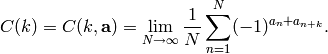
In the case where is periodic with period
 then this reduces to
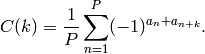
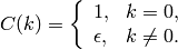
Assume is periodic with period .
balance: 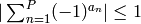 .
.
low autocorrelation:
(For sequences satisfying these first two properties, it is known
that  must hold.)
proportional runs property: In each period, half the runs have
length  , one-fourth have length
  , etc.
Moreover, there are as many runs of ‘s as there are of
, etc.
Moreover, there are as many runs of ‘s as there are of
 ‘s.
‘s.
A general feedback shift register is a map
 of the form
where  is a given
function. When
is a given
function. When  is of the form

for some given constants  , the map is
called a linear feedback shift register (LFSR).
, the map is
called a linear feedback shift register (LFSR).
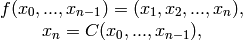
Example of a LFSR Let


be given polynomials in ![{\bf F}_2[x]](../../_images/math/811f707e42cead2b2236dd3a535d3bfa2fa3ae44.png) and let
and let
We can compute a recursion formula which allows us to rapidly
compute the coefficients of  (take
(take  ):
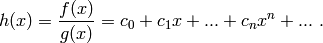
):
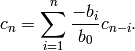
The coefficients of can, under certain conditions on
 and
and  , be considered “random” from
certain statistical points of view.
, be considered “random” from
certain statistical points of view.
Example: For instance, if

then

The coefficients of  are
are
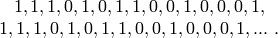
The sequence of  ‘s is periodic with period
 and satisfies Golomb’s three randomness
conditions. However, this sequence of period 15 can be “cracked”
(i.e., a procedure to reproduce ) by knowing only 8
terms! This is the function of the Berlekamp-Massey algorithm [M],
implemented as berlekamp_massey.py.
and satisfies Golomb’s three randomness
conditions. However, this sequence of period 15 can be “cracked”
(i.e., a procedure to reproduce ) by knowing only 8
terms! This is the function of the Berlekamp-Massey algorithm [M],
implemented as berlekamp_massey.py.
| [G] | Solomon Golomb, Shift register sequences, Aegean Park Press, Laguna Hills, Ca, 1967 |
| [M] | (1, 2) James L. Massey, “Shift-Register Synthesis and BCH Decoding.” IEEE Trans. on Information Theory, vol. 15(1), pp. 122-127, Jan 1969. |
AUTHORS:
Created 11-24-2005 by wdj. Last updated 12-02-2005.
INPUT:
OUTPUT: autocorrelation sequence of L
EXAMPLES:
sage: F = GF(2)
sage: o = F(0)
sage: l = F(1)
sage: key = [l,o,o,l]; fill = [l,l,o,l]; n = 20
sage: s = lfsr_sequence(key,fill,n)
sage: lfsr_autocorrelation(s,15,7)
4/15
sage: lfsr_autocorrelation(s,int(15),7)
4/15
AUTHORS:
INPUT:
OUTPUT:
This implements the algorithm in section 3 of J. L. Massey’s article [M].
EXAMPLE:
sage: F = GF(2)
sage: F
Finite Field of size 2
sage: o = F(0); l = F(1)
sage: key = [l,o,o,l]; fill = [l,l,o,l]; n = 20
sage: s = lfsr_sequence(key,fill,n); s
[1, 1, 0, 1, 0, 1, 1, 0, 0, 1, 0, 0, 0, 1, 1, 1, 1, 0, 1, 0]
sage: lfsr_connection_polynomial(s)
x^4 + x + 1
sage: berlekamp_massey(s)
x^4 + x^3 + 1
Notice that berlekamp_massey returns the reverse of the connection polynomial (and is potentially must faster than this implementation).
AUTHORS:
This function creates an lfsr sequence.
INPUT:
OUTPUT: The lfsr sequence defined by
 , for
, for
 .
.
EXAMPLES:
sage: F = GF(2); l = F(1); o = F(0)
sage: F = GF(2); S = LaurentSeriesRing(F,'x'); x = S.gen()
sage: fill = [l,l,o,l]; key = [1,o,o,l]; n = 20
sage: L = lfsr_sequence(key,fill,20); L
[1, 1, 0, 1, 0, 1, 1, 0, 0, 1, 0, 0, 0, 1, 1, 1, 1, 0, 1, 0]
sage: g = berlekamp_massey(L); g
x^4 + x^3 + 1
sage: (1)/(g.reverse()+O(x^20))
1 + x + x^2 + x^3 + x^5 + x^7 + x^8 + x^11 + x^15 + x^16 + x^17 + x^18 + O(x^20)
sage: (1+x^2)/(g.reverse()+O(x^20))
1 + x + x^4 + x^8 + x^9 + x^10 + x^11 + x^13 + x^15 + x^16 + x^19 + O(x^20)
sage: (1+x^2+x^3)/(g.reverse()+O(x^20))
1 + x + x^3 + x^5 + x^6 + x^9 + x^13 + x^14 + x^15 + x^16 + x^18 + O(x^20)
sage: fill = [l,l,o,l]; key = [l,o,o,o]; n = 20
sage: L = lfsr_sequence(key,fill,20); L
[1, 1, 0, 1, 1, 1, 0, 1, 1, 1, 0, 1, 1, 1, 0, 1, 1, 1, 0, 1]
sage: g = berlekamp_massey(L); g
x^4 + 1
sage: (1+x)/(g.reverse()+O(x^20))
1 + x + x^4 + x^5 + x^8 + x^9 + x^12 + x^13 + x^16 + x^17 + O(x^20)
sage: (1+x+x^3)/(g.reverse()+O(x^20))
1 + x + x^3 + x^4 + x^5 + x^7 + x^8 + x^9 + x^11 + x^12 + x^13 + x^15 + x^16 + x^17 + x^19 + O(x^20)
AUTHORS: