Solving ordinary differential equations¶

This file contains functions useful for solving differential equations which occur commonly in a 1st semester differential equations course. For another numerical solver see ode_solver() function and optional package Octave.

Commands:

desolve - Computes the “general solution” to a 1st or 2nd order ODE via Maxima.
desolve_laplace - Solves an ODE using laplace transforms via Maxima. Initials conditions are optional.
desolve_system - Solves any size system of 1st order odes using Maxima. Initials conditions are optional.
desolve_rk4 - Solves numerically IVP for one first order equation, returns list of points or plot
desolve_system_rk4 - Solves numerically IVP for system of first order equations, returns list of points
eulers_method - Approximate solution to a 1st order DE, presented as a table.
eulers_method_2x2 - Approximate solution to a 1st order system of DEs, presented as a table.
eulers_method_2x2_plot - Plots the sequence of points obtained from Euler’s method.

AUTHORS:

David Joyner (3-2006) - Initial version of functions
Marshall Hampton (7-2007) - Creation of Python module and testing
Robert Bradshaw (10-2008) - Some interface cleanup.
Robert Marik (10-2009) - Some bugfixes and enhancements

sage.calculus.desolvers.desolve(de, dvar, ics=None, ivar=None, show_method=False, contrib_ode=False)¶

Solves a 1st or 2nd order linear ODE via maxima. Including IVP and BVP.

Use desolve? <tab> if the output in truncated in notebook.

INPUT:

de - an expression or equation representing the ODE
dvar - the dependent variable (hereafter called y)
ics - (optional) the initial or boundary conditions
- for a first-order equation, specify the initial x and y
- for a second-order equation, specify the initial x, y, and dy/dx
- for a second-order boundary solution, specify initial and final x and y initial conditions gives error if the solution is not SymbolicEquation (as happens for example for clairot equation)
ivar - (optional) the independent variable (hereafter called x), which must be specified if there is more than one independent variable in the equation.
show_method - (optional) if true, then Sage returns pair [solution, method], where method is the string describing method which has been used to get solution (Maxima uses the following order for first order equations: linear, separable, exact (including exact with integrating factor), homogeneous, bernoulli, generalized homogeneous) - use carefully in class, see below for the example of the equation which is separable but this property is not recognized by Maxima and equation is solved as exact.
contrib_ode - (optional) if true, desolve allows to solve clairot, lagrange, riccati and some other equations. May take a long time and thus turned off by default. Initial conditions can be used only if the result is one SymbolicEquation (does not contain singular solution, for example)

OUTPUT:

In most cases returns SymbolicEquation which defines the solution implicitly. If the result is in the form y(x)=... (happens for linear eqs.), returns the right-hand side only. The possible constant solutions of separable ODE’s are omitted.

EXAMPLES:

sage: x = var('x')
sage: y = function('y', x)
sage: desolve(diff(y,x) + y - 1, y)
(c + e^x)*e^(-x)

sage: f = desolve(diff(y,x) + y - 1, y, ics=[10,2]); f
(e^10 + e^x)*e^(-x)

sage: plot(f)

We can also solve second-order differential equations.:

sage: x = var('x')
sage: y = function('y', x)
sage: de = diff(y,x,2) - y == x
sage: desolve(de, y)
k1*e^x + k2*e^(-x) - x

sage: f = desolve(de, y, [10,2,1]); f
-x + 5*e^(-x + 10) + 7*e^(x - 10)
sage: f(x=10)
2
sage: diff(f,x)(x=10)
1

sage: de = diff(y,x,2) + y == 0
sage: desolve(de, y)
k1*sin(x) + k2*cos(x)
sage: desolve(de, y, [0,1,pi/2,4]) 
4*sin(x) + cos(x)

sage: desolve(y*diff(y,x)+sin(x)==0,y)
-1/2*y(x)^2 == c - cos(x)

Clairot equation: general and singular solutions:

sage: desolve(diff(y,x)^2+x*diff(y,x)-y==0,y,contrib_ode=True,show_method=True)
[[y(x) == c^2 + c*x, y(x) == -1/4*x^2], 'clairault']

For equations involving more variables we specify independent variable:

sage: a,b,c,n=var('a b c n')
sage: desolve(x^2*diff(y,x)==a+b*x^n+c*x^2*y^2,y,ivar=x,contrib_ode=True)
[[y(x) == 0, (b*x^(n - 2) + a/x^2)*c^2*u == 0]]
sage: desolve(x^2*diff(y,x)==a+b*x^n+c*x^2*y^2,y,ivar=x,contrib_ode=True,show_method=True)
[[[y(x) == 0, (b*x^(n - 2) + a/x^2)*c^2*u == 0]], 'riccati']

Higher orded, not involving independent variable:

sage: desolve(diff(y,x,2)+y*(diff(y,x,1))^3==0,y).expand()
1/6*y(x)^3 + k1*y(x) == k2 + x
sage: desolve(diff(y,x,2)+y*(diff(y,x,1))^3==0,y,[0,1,1,3]).expand()
1/6*y(x)^3 - 5/3*y(x) == x - 3/2
sage: desolve(diff(y,x,2)+y*(diff(y,x,1))^3==0,y,[0,1,1,3],show_method=True)
[1/6*y(x)^3 - 5/3*y(x) == x - 3/2, 'freeofx']

Separable equations - Sage returns solution in implicit form:

sage: desolve(diff(y,x)*sin(y) == cos(x),y)
-cos(y(x)) == c + sin(x)
sage: desolve(diff(y,x)*sin(y) == cos(x),y,show_method=True)
[-cos(y(x)) == c + sin(x), 'separable']
sage: desolve(diff(y,x)*sin(y) == cos(x),y,[pi/2,1])
-cos(y(x)) == sin(x) - cos(1) - 1

Linear equation - Sage returns the expression on the right hand side only:

sage: desolve(diff(y,x)+(y) == cos(x),y)
1/2*((sin(x) + cos(x))*e^x + 2*c)*e^(-x)
sage: desolve(diff(y,x)+(y) == cos(x),y,show_method=True)
[1/2*((sin(x) + cos(x))*e^x + 2*c)*e^(-x), 'linear']
sage: desolve(diff(y,x)+(y) == cos(x),y,[0,1])
1/2*(e^x*sin(x) + e^x*cos(x) + 1)*e^(-x)

This ODE with separated variables is solved as exact. Explanation - factor does not split $e^{x-y}$ in Maxima into $e^{x}e^{y}$ :

sage: desolve(diff(y,x)==exp(x-y),y,show_method=True)
[-e^x + e^y(x) == c, 'exact']

You can solve Bessel equations. You can also use initial conditions, but you cannot put (sometimes desired) initial condition at x=0, since this point is singlar point of the equation. Anyway, if the solution should be bounded at x=0, then k2=0.:

sage: desolve(x^2*diff(y,x,x)+x*diff(y,x)+(x^2-4)*y==0,y)
k1*bessel_j(2, x) + k2*bessel_y(2, x)

Difficult ODE produces error:

sage: desolve(sqrt(y)*diff(y,x)+e^(y)+cos(x)-sin(x+y)==0,y) # not tested
Traceback (click to the left for traceback)
...
NotImplementedError, "Maxima was unable to solve this ODE. Consider to set option contrib_ode to True."

Difficult ODE produces error - moreover, takes a long time

sage: desolve(sqrt(y)*diff(y,x)+e^(y)+cos(x)-sin(x+y)==0,y,contrib_ode=True) # not tested

Some more types od ODE’s:

sage: desolve(x*diff(y,x)^2-(1+x*y)*diff(y,x)+y==0,y,contrib_ode=True,show_method=True)
[[y(x) == c + log(x), y(x) == c*e^x], 'factor']

sage: desolve(diff(y,x)==(x+y)^2,y,contrib_ode=True,show_method=True)
[[[x == c - arctan(sqrt(t)), y(x) == -x - sqrt(t)], [x == c + arctan(sqrt(t)), y(x) == -x + sqrt(t)]], 'lagrange']

These two examples produce error (as expected, Maxima 5.18 cannot solve equations from initial conditions). Current Maxima 5.18 returns false answer in this case!:

sage: desolve(diff(y,x,2)+y*(diff(y,x,1))^3==0,y,[0,1,2]).expand() # not tested
Traceback (click to the left for traceback)
...
NotImplementedError, "Maxima was unable to solve this ODE. Consider to set option contrib_ode to True."

sage: desolve(diff(y,x,2)+y*(diff(y,x,1))^3==0,y,[0,1,2],show_method=True) # not tested
Traceback (click to the left for traceback)
...
NotImplementedError, "Maxima was unable to solve this ODE. Consider to set option contrib_ode to True."

Second order linear ODE:

sage: desolve(diff(y,x,2)+2*diff(y,x)+y == cos(x),y)
(k2*x + k1)*e^(-x) + 1/2*sin(x)
sage: desolve(diff(y,x,2)+2*diff(y,x)+y == cos(x),y,show_method=True)
[(k2*x + k1)*e^(-x) + 1/2*sin(x), 'variationofparameters']
sage: desolve(diff(y,x,2)+2*diff(y,x)+y == cos(x),y,[0,3,1])
1/2*(7*x + 6)*e^(-x) + 1/2*sin(x)
sage: desolve(diff(y,x,2)+2*diff(y,x)+y == cos(x),y,[0,3,1],show_method=True)
[1/2*(7*x + 6)*e^(-x) + 1/2*sin(x), 'variationofparameters']
sage: desolve(diff(y,x,2)+2*diff(y,x)+y == cos(x),y,[0,3,pi/2,2])
3*((e^(1/2*pi) - 2)*x/pi + 1)*e^(-x) + 1/2*sin(x)
sage: desolve(diff(y,x,2)+2*diff(y,x)+y == cos(x),y,[0,3,pi/2,2],show_method=True)
[3*((e^(1/2*pi) - 2)*x/pi + 1)*e^(-x) + 1/2*sin(x), 'variationofparameters']

sage: desolve(diff(y,x,2)+2*diff(y,x)+y == 0,y)
(k2*x + k1)*e^(-x)
sage: desolve(diff(y,x,2)+2*diff(y,x)+y == 0,y,show_method=True)
[(k2*x + k1)*e^(-x), 'constcoeff']
sage: desolve(diff(y,x,2)+2*diff(y,x)+y == 0,y,[0,3,1])
(4*x + 3)*e^(-x)
sage: desolve(diff(y,x,2)+2*diff(y,x)+y == 0,y,[0,3,1],show_method=True)
[(4*x + 3)*e^(-x), 'constcoeff']
sage: desolve(diff(y,x,2)+2*diff(y,x)+y == 0,y,[0,3,pi/2,2])
(2*(2*e^(1/2*pi) - 3)*x/pi + 3)*e^(-x)
sage: desolve(diff(y,x,2)+2*diff(y,x)+y == 0,y,[0,3,pi/2,2],show_method=True)
[(2*(2*e^(1/2*pi) - 3)*x/pi + 3)*e^(-x), 'constcoeff']

This equation can be solved within Maxima but not within Sage. It needs assumptions assume(x>0,y>0) and works in Maxima, but not in Sage:

sage: assume(x>0) # not tested
sage: assume(y>0) # not tested
sage: desolve(x*diff(y,x)-x*sqrt(y^2+x^2)-y,y,show_method=True) # not tested

TESTS:

Trac #6479 fixed:

sage: x = var('x')
sage: y = function('y', x)
sage: desolve( diff(y,x,x) == 0, y, [0,0,1])
x

sage: desolve( diff(y,x,x) == 0, y, [0,1,1])
x + 1

AUTHORS:

David Joyner (1-2006)
Robert Bradshaw (10-2008)
Robert Marik (10-2009)

sage.calculus.desolvers.desolve_laplace(de, dvar, ics=None, ivar=None)¶

Solves an ODE using laplace transforms. Initials conditions are optional.

INPUT:

de - a lambda expression representing the ODE (eg, de = diff(y,x,2) == diff(y,x)+sin(x))
dvar - the dependent variable (eg y)
ivar - (optional) the independent variable (hereafter called x), which must be specified if there is more than one independent variable in the equation.
ics - a list of numbers representing initial conditions, (eg, f(0)=1, f’(0)=2 is ics = [0,1,2])

OUTPUT:

Solution of the ODE as symbolic expression

EXAMPLES:

sage: u=function('u',x)
sage: eq = diff(u,x) - exp(-x) - u == 0
sage: desolve_laplace(eq,u)
1/2*(2*u(0) + 1)*e^x - 1/2*e^(-x)

We can use initial conditions:

sage: desolve_laplace(eq,u,ics=[0,3])
-1/2*e^(-x) + 7/2*e^x

The initial conditions do not persist in the system (as they persisted in previous versions):

sage: desolve_laplace(eq,u)
1/2*(2*u(0) + 1)*e^x - 1/2*e^(-x)

sage: f=function('f', x)
sage: eq = diff(f,x) + f == 0
sage: desolve_laplace(eq,f,[0,1])
e^(-x)

sage: x = var('x')
sage: f = function('f', x)
sage: de = diff(f,x,x) - 2*diff(f,x) + f
sage: desolve_laplace(de,f)
-x*e^x*f(0) + x*e^x*D[0](f)(0) + e^x*f(0)
sage: desolve_laplace(de,f,ics=[0,1,2])
x*e^x + e^x

TESTS:

Trac #4839 fixed:

sage: t=var('t')
sage: x=function('x', t)
sage: soln=desolve_laplace(diff(x,t)+x==1, x, ics=[0,2])
sage: soln
e^(-t) + 1
sage: soln(t=3)
e^(-3) + 1

AUTHORS:

David Joyner (1-2006,8-2007)
Robert Marik (10-2009)

sage.calculus.desolvers.desolve_rk4(de, dvar, ics=None, ivar=None, end_points=None, step=0.10000000000000001, output='list', **kwds)¶

Solves numerically one first-order ordinary differential equation. See also ode_solver.

INPUT:

input is similar to desolve command. The differential equation can be written in a form close to the plot_slope_field or desolve command

Variant 1 (function in two variables)
- de - right hand side, i.e. the function $f(x,y)$ from ODE $y'=f(x,y)$
- dvar - dependent variable (symbolic variable declared by var)
Variant 2 (symbolic equation)
- de - equation, including term with diff(y,x)
- dvar` - dependent variable (declared as funciton of independent variable)
Other parameters
- ivar - should be specified, if there are more variables or if the equation is autonomous
- ics - initial conditions in the form [x0,y0]
- end_points - the end points of the interval
  - if end_points is a or [a], we integrate on between min(ics[0],a) and max(ics[0],a)
  - if end_points is None, we use end_points=ics[0]+10
  - if end_points is [a,b] we integrate on between min(ics[0],a) and max(ics[0],b)
- step - (optional, default:0.1) the length of the step (positive number)
- output - (optional, default: ‘list’) one of ‘list’, ‘plot’, ‘slope_field’ (graph of the solution with slope field)

OUTPUT:

Returns a list of points, or plot produced by list_plot, optionally with slope field.

EXAMPLES:

sage: from sage.calculus.desolvers import desolve_rk4

Variant 2 for input - more common in numerics:

sage: x,y=var('x y')
sage: desolve_rk4(x*y*(2-y),y,ics=[0,1],end_points=1,step=0.5)
[[0, 1], [0.5, 1.12419127425], [1.0, 1.46159016229]]

Variant 1 for input - we can pass ODE in the form used by desolve function In this example we integrate bakwards, since end_points < ics[0]:

sage: y=function('y',x) 
sage: desolve_rk4(diff(y,x)+y*(y-1) == x-2,y,ics=[1,1],step=0.5, end_points=0) 
[[0.0, 8.90425710896], [0.5, 1.90932794536], [1, 1]]

Here we show how to plot simple pictures. For more advanced aplications use list_plot instead. To see the resulting picture use show(P) in Sage notebook.

sage: x,y=var('x y')
sage: P=desolve_rk4(y*(2-y),y,ics=[0,.1],ivar=x,output='slope_field',end_points=[-4,6],thickness=3)

ALGORITHM:

4th order Runge-Kutta method. Wrapper for command rk in Maxima’s dynamics package. Perhaps could be faster by using fast_float instead.

AUTHORS:

Robert Marik (10-2009)

sage.calculus.desolvers.desolve_rk4_determine_bounds(ics, end_points=None)¶

Used to determine bounds for numerical integration.

If end_points is None, the interval for integration is from ics[0] to ics[0]+10
If end_points is a or [a], the interval for integration is from min(ics[0],a) to max(ics[0],a)
If end_points is [a,b], the interval for integration is from min(ics[0],a) to max(ics[0],b)

EXAMPLES:

sage: from sage.calculus.desolvers import desolve_rk4_determine_bounds
sage: desolve_rk4_determine_bounds([0,2],1)
(0, 1)

sage: desolve_rk4_determine_bounds([0,2])  
(0, 10)

sage: desolve_rk4_determine_bounds([0,2],[-2])
(-2, 0)

sage: desolve_rk4_determine_bounds([0,2],[-2,4])
(-2, 4)

sage.calculus.desolvers.desolve_system(des, vars, ics=None, ivar=None)¶

Solves any size system of 1st order ODE’s. Initials conditions are optional.

INPUT:

des - list of ODEs
vars - list of dependent variables
ics - (optional) list of initial values for ivar and vars
ivar - (optional) the independent variable, which must be specified if there is more than one independent variable in the equation.

EXAMPLES:

sage: t = var('t')
sage: x = function('x', t)
sage: y = function('y', t)
sage: de1 = diff(x,t) + y - 1 == 0
sage: de2 = diff(y,t) - x + 1 == 0
sage: desolve_system([de1, de2], [x,y])
[x(t) == (x(0) - 1)*cos(t) - (y(0) - 1)*sin(t) + 1,
 y(t) == (x(0) - 1)*sin(t) + (y(0) - 1)*cos(t) + 1]

Now we give some initial conditions:

sage: sol = desolve_system([de1, de2], [x,y], ics=[0,1,2]); sol
[x(t) == -sin(t) + 1, y(t) == cos(t) + 1]
sage: solnx, solny = sol[0].rhs(), sol[1].rhs()
sage: plot([solnx,solny],(0,1))
sage: parametric_plot((solnx,solny),(0,1))

AUTHORS:

Robert Bradshaw (10-2008)

sage.calculus.desolvers.desolve_system_rk4(des, vars, ics=None, ivar=None, end_points=None, step=0.10000000000000001)¶

Solves numerically system of first-order ordinary differential equations using the 4th order Runge-Kutta method. Wrapper for Maxima command rk. See also ode_solver.

INPUT:

input is similar to desolve_system and desolve_rk4 commands

des - right hand sides of the system
vars - dependent variables
ivar - (optional) should be specified, if there are more variables or if the equation is autonomous and the independent variable is missing
ics - initial conditions in the form [x0,y01,y02,y03,....]
end_points - the end points of the interval
- if end_points is a or [a], we integrate on between min(ics[0],a) and max(ics[0],a)
- if end_points is None, we use end_points=ics[0]+10
- if end_points is [a,b] we integrate on between min(ics[0],a) and max(ics[0],b)
step – (optional, default: 0.1) the length of the step

OUTPUT:

Returns a list of points.

EXAMPLES:

sage: from sage.calculus.desolvers import desolve_system_rk4

Lotka Volterra system:

sage: from sage.calculus.desolvers import desolve_system_rk4
sage: x,y,t=var('x y t')
sage: P=desolve_system_rk4([x*(1-y),-y*(1-x)],[x,y],ics=[0,0.5,2],ivar=t,end_points=20)
sage: Q=[ [i,j] for i,j,k in P]
sage: LP=list_plot(Q)

sage: Q=[ [j,k] for i,j,k in P]
sage: LP=list_plot(Q)

ALGORITHM:

4th order Runge-Kutta method. Wrapper for command rk in Maxima’s dynamics package. Perhaps could be faster by using fast_float instead.

AUTHOR:

Robert Marik (10-2009)

sage.calculus.desolvers.desolve_system_strings(des, vars, ics=None)¶

Solves any size system of 1st order ODE’s. Initials conditions are optional.

This function is obsolete, use desolve_system.

INPUT:

de - a list of strings representing the ODEs in maxima notation (eg, de = “diff(f(x),x,2)=diff(f(x),x)+sin(x)”)
vars - a list of strings representing the variables (eg, vars = [“s”,”x”,”y”], where s is the independent variable and x,y the dependent variables)
ics - a list of numbers representing initial conditions (eg, x(0)=1, y(0)=2 is ics = [0,1,2])

WARNING:

The given ics sets the initial values of the dependent vars in maxima, so subsequent ODEs involving these variables will have these initial conditions automatically imposed.

EXAMPLES:

sage: from sage.calculus.desolvers import desolve_system_strings
sage: s = var('s')
sage: function('x', s)
x(s)
sage: function('y', s)
y(s)
sage: de1 = lambda z: diff(z[0],s) + z[1] - 1
sage: de2 = lambda z: diff(z[1],s) - z[0] + 1
sage: des = [de1([x(s),y(s)]),de2([x(s),y(s)])]
sage: vars = ["s","x","y"]
sage: desolve_system_strings(des,vars)
["(1-'y(0))*sin(s)+('x(0)-1)*cos(s)+1", "('x(0)-1)*sin(s)+('y(0)-1)*cos(s)+1"]
sage: ics = [0,1,-1]
sage: soln = desolve_system_strings(des,vars,ics); soln
['2*sin(s)+1', '1-2*cos(s)']
sage: solnx, solny = map(SR, soln)
sage: RR(solnx(s=3))
1.28224001611973
sage: P1 = plot([solnx,solny],(0,1))
sage: P2 = parametric_plot((solnx,solny),(0,1))

Now type show(P1), show(P2) to view these.

AUTHORS:

David Joyner (3-2006, 8-2007)

sage.calculus.desolvers.eulers_method(f, x0, y0, h, x1, method='table')¶

This implements Euler’s method for finding numerically the solution of the 1st order ODE y' = f(x,y), y(a)=c. The “x” column of the table increments from x0 to x1 by h (so (x1-x0)/h must be an integer). In the “y” column, the new y-value equals the old y-value plus the corresponding entry in the last column.

For pedagogical purposes only.

EXAMPLES:

sage: from sage.calculus.desolvers import eulers_method
sage: x,y = PolynomialRing(QQ,2,"xy").gens()
sage: eulers_method(5*x+y-5,0,1,1/2,1)
     x                    y                  h*f(x,y)
     0                    1                   -2
   1/2                   -1                 -7/4
     1                -11/4                -11/8

sage: x,y = PolynomialRing(QQ,2,"xy").gens()
sage: eulers_method(5*x+y-5,0,1,1/2,1,method="none")
[[0, 1], [1/2, -1], [1, -11/4], [3/2, -33/8]]

sage: RR = RealField(sci_not=0, prec=4, rnd='RNDU')
sage: x,y = PolynomialRing(RR,2,"xy").gens()
sage: eulers_method(5*x+y-5,0,1,1/2,1,method="None")
[[0, 1], [1/2, -1.0], [1, -2.7], [3/2, -4.0]]

sage: RR = RealField(sci_not=0, prec=4, rnd='RNDU')
sage: x,y=PolynomialRing(RR,2,"xy").gens()
sage: eulers_method(5*x+y-5,0,1,1/2,1)
     x                    y                  h*f(x,y)
     0                    1                 -2.0
   1/2                 -1.0                 -1.7
     1                 -2.7                 -1.3

sage: x,y=PolynomialRing(QQ,2,"xy").gens()
sage: eulers_method(5*x+y-5,1,1,1/3,2)
         x                    y                  h*f(x,y)
         1                    1                  1/3
       4/3                  4/3                    1
       5/3                  7/3                 17/9
         2                 38/9                83/27

sage: eulers_method(5*x+y-5,0,1,1/2,1,method="none")
[[0, 1], [1/2, -1], [1, -11/4], [3/2, -33/8]]

sage: pts = eulers_method(5*x+y-5,0,1,1/2,1,method="none")
sage: P1 = list_plot(pts)
sage: P2 = line(pts)
sage: (P1+P2).show()

AUTHORS:

David Joyner

sage.calculus.desolvers.eulers_method_2x2(f, g, t0, x0, y0, h, t1, method='table')¶

This implements Euler’s method for finding numerically the solution of the 1st order system of two ODEs

x' = f(t, x, y), x(t0)=x0.

y' = g(t, x, y), y(t0)=y0.

The “t” column of the table increments from $t_0$ to $t_1$ by $h$ (so $\\frac{t_1-t_0}{h}$ must be an integer). In the “x” column, the new x-value equals the old x-value plus the corresponding entry in the next (third) column. In the “y” column, the new y-value equals the old y-value plus the corresponding entry in the next (last) column.

For pedagogical purposes only.

EXAMPLES:

sage: from sage.calculus.desolvers import eulers_method_2x2
sage: t, x, y = PolynomialRing(QQ,3,"txy").gens()
sage: f = x+y+t; g = x-y
sage: eulers_method_2x2(f,g, 0, 0, 0, 1/3, 1,method="none")
[[0, 0, 0], [1/3, 0, 0], [2/3, 1/9, 0], [1, 10/27, 1/27], [4/3, 68/81, 4/27]]

sage: eulers_method_2x2(f,g, 0, 0, 0, 1/3, 1)
     t                    x                h*f(t,x,y)                    y           h*g(t,x,y)
     0                    0                         0                    0                    0
   1/3                    0                       1/9                    0                    0
   2/3                  1/9                      7/27                    0                 1/27
     1                10/27                     38/81                 1/27                  1/9

sage: RR = RealField(sci_not=0, prec=4, rnd='RNDU')
sage: t,x,y=PolynomialRing(RR,3,"txy").gens()
sage: f = x+y+t; g = x-y
sage: eulers_method_2x2(f,g, 0, 0, 0, 1/3, 1)
     t                    x                h*f(t,x,y)                    y           h*g(t,x,y)
     0                    0                      0.00                    0                 0.00
   1/3                 0.00                      0.13                 0.00                 0.00
   2/3                 0.13                      0.29                 0.00                0.043
     1                 0.41                      0.57                0.043                 0.15

To numerically approximate $y(1)$ , where $(1+t^2)y''+y'-y=0$ , $y(0)=1$ , $y'(0)=-1$ , using 4 steps of Euler’s method, first convert to a system: $y_1' = y_2$ , $y_1(0)=1$ ; $y_2' = \\frac{y_1-y_2}{1+t^2}$ , $y_2(0)=-1$ .:

sage: RR = RealField(sci_not=0, prec=4, rnd='RNDU')
sage: t, x, y=PolynomialRing(RR,3,"txy").gens()
sage: f = y; g = (x-y)/(1+t^2)
sage: eulers_method_2x2(f,g, 0, 1, -1, 1/4, 1)
    t                    x                h*f(t,x,y)                    y           h*g(t,x,y)
    0                    1                     -0.25                   -1                 0.50
  1/4                 0.75                     -0.12                -0.50                 0.29
  1/2                 0.63                    -0.054                -0.21                 0.19
  3/4                 0.63                   -0.0078               -0.031                 0.11
    1                 0.63                     0.020                0.079                0.071

To numerically approximate y(1), where $y''+ty'+y=0$ , $y(0)=1$ , $y'(0)=0$ :

sage: t,x,y=PolynomialRing(RR,3,"txy").gens()
sage: f = y; g = -x-y*t
sage: eulers_method_2x2(f,g, 0, 1, 0, 1/4, 1)
     t                    x                h*f(t,x,y)                    y           h*g(t,x,y)
     0                    1                      0.00                    0                -0.25
   1/4                  1.0                    -0.062                -0.25                -0.23
   1/2                 0.94                     -0.11                -0.46                -0.17
   3/4                 0.88                     -0.15                -0.62                -0.10
     1                 0.75                     -0.17                -0.68               -0.015

AUTHORS:

David Joyner

sage.calculus.desolvers.eulers_method_2x2_plot(f, g, t0, x0, y0, h, t1)¶

Plots solution of ODE

This plots the soln in the rectangle (xrange[0],xrange[1]) x (yrange[0],yrange[1]) and plots using Euler’s method the numerical solution of the 1st order ODEs $x' = f(t,x,y)$ , $x(a)=x_0$ , $y' = g(t,x,y)$ , $y(a) = y_0$ .

For pedagogical purposes only.

EXAMPLES:

sage: from sage.calculus.desolvers import eulers_method_2x2_plot

The following example plots the solution to 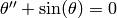$\theta''+\sin(\theta)=0$ , $\theta(0)=\frac 34$ , $\theta'(0) = 0$ . Type P[0].show() to plot the solution, (P[0]+P[1]).show() to plot $(t,\theta(t))$ and $(t,\theta'(t))$ :

sage: f = lambda z : z[2]; g = lambda z : -sin(z[1])
sage: P = eulers_method_2x2_plot(f,g, 0.0, 0.75, 0.0, 0.1, 1.0)

Solving ordinary differential equations¶

Previous topic

Next topic

This Page

Navigation

Solving ordinary differential equations¶

Previous topic

Next topic

This Page

Quick search

Navigation