AUTHORS:
This package defines functions for computing various bases of the Steenrod algebra, and for converting between the Milnor basis and any other basis.
This packages implements a number of different bases, at least at the prime 2. The Milnor and Serre-Cartan bases are the most familiar and most standard ones, and all of the others are defined in terms of one of these. The bases are described in the documentation for the function steenrod_algebra_basis; also see the papers by Monks [M] and Wood [W] for more information about them. For commutator bases, see the preprint by Palmieri and Zhang [PZ].
The other bases are as follows; these are only defined when
 :
:
 -bases.
EXAMPLES:
sage: steenrod_algebra_basis(7,'milnor')
(Sq(0,0,1), Sq(1,2), Sq(4,1), Sq(7))
sage: steenrod_algebra_basis(5)   # milnor basis is the default
(Sq(2,1), Sq(5))
The third (optional) argument to
steenrod_algebra_basis is the prime  :
:
sage: steenrod_algebra_basis(9, 'milnor', p=3)
(Q_1 P(1), Q_0 P(2))
sage: steenrod_algebra_basis(9, 'milnor', 3)
(Q_1 P(1), Q_0 P(2))
sage: steenrod_algebra_basis(17, 'milnor', 3)
(Q_2, Q_1 P(3), Q_0 P(0,1), Q_0 P(4))
Other bases:
sage: steenrod_algebra_basis(7,'admissible')
(Sq^{7}, Sq^{6} Sq^{1}, Sq^{4} Sq^{2} Sq^{1}, Sq^{5} Sq^{2})
sage: [x.basis('milnor') for x in steenrod_algebra_basis(7,'admissible')]
[Sq(7),
Sq(4,1) + Sq(7),
Sq(0,0,1) + Sq(1,2) + Sq(4,1) + Sq(7),
Sq(1,2) + Sq(7)]
sage: Aw = SteenrodAlgebra(2, basis = 'wall_long')
sage: [Aw(x) for x in steenrod_algebra_basis(7,'admissible')]
[Sq^{1} Sq^{2} Sq^{4},
Sq^{2} Sq^{4} Sq^{1},
Sq^{4} Sq^{2} Sq^{1},
Sq^{4} Sq^{1} Sq^{2}]
sage: steenrod_algebra_basis(13,'admissible',p=3)
(beta P^{3}, P^{3} beta)
sage: steenrod_algebra_basis(5,'wall')
(Q^{2}_{2} Q^{0}_{0}, Q^{1}_{1} Q^{1}_{0})
sage: steenrod_algebra_basis(5,'wall_long')
(Sq^{4} Sq^{1}, Sq^{2} Sq^{1} Sq^{2})
sage: steenrod_algebra_basis(5,'pst-rlex')
(P^{0}_{1} P^{2}_{1}, P^{1}_{1} P^{0}_{2})
This file also contains a function milnor_convert
which converts elements from the (default) Milnor basis
representation to a representation in another basis. The output is
a dictionary which gives the new representation; its form depends
on the chosen basis. For example, in the basis of admissible
sequences (a.k.a. the Serre-Cartan basis), each basis element is of
the form  , and so is
represented by a tuple
, and so is
represented by a tuple  of integers. Thus the
dictionary has such tuples as keys, with the coefficient of the
basis element as the associated value:
of integers. Thus the
dictionary has such tuples as keys, with the coefficient of the
basis element as the associated value:
sage: from sage.algebras.steenrod_algebra_bases import milnor_convert
sage: milnor_convert(Sq(2)*Sq(4) + Sq(2)*Sq(5), 'admissible')
{(5, 1): 1, (6, 1): 1, (6,): 1}
sage: milnor_convert(Sq(2)*Sq(4) + Sq(2)*Sq(5), 'pst')
{((1, 1), (2, 1)): 1, ((0, 1), (1, 1), (2, 1)): 1, ((0, 2), (2, 1)): 1}
Users shouldn’t need to call milnor_convert; they should use the basis method to view a single element in another basis, or define a Steenrod algebra with a different default basis and work in that algebra:
sage: x = Sq(2)*Sq(4) + Sq(2)*Sq(5)
sage: x
Sq(3,1) + Sq(4,1) + Sq(6) + Sq(7)
sage: x.basis('milnor')  # 'milnor' is the default basis
Sq(3,1) + Sq(4,1) + Sq(6) + Sq(7)
sage: x.basis('adem')
Sq^{5} Sq^{1} + Sq^{6} + Sq^{6} Sq^{1}
sage: x.basis('pst')
P^{0}_{1} P^{1}_{1} P^{2}_{1} + P^{0}_{2} P^{2}_{1} + P^{1}_{1} P^{2}_{1}
sage: A = SteenrodAlgebra(2, basis='pst')
sage: A(Sq(2) * Sq(4) + Sq(2) * Sq(5))
P^{0}_{1} P^{1}_{1} P^{2}_{1} + P^{0}_{2} P^{2}_{1} + P^{1}_{1} P^{2}_{1}
INTERNAL DOCUMENTATION:
If you want to implement a new basis for the Steenrod algebra:
In the file ‘steenrod_algebra.py’:
In the file ‘steenrod_algebra_element.py’:
In this file ‘steenrod_algebra_bases.py’:
REFERENCES:
bases for the Steenrod algebra,” J. Pure Appl.
Algebra 125 (1998), no. 1-3, 235-260.Compute  (Wall basis) and
  (Arnon’s
A basis).
(Arnon’s
A basis).
INPUT:

OUTPUT: element of Steenrod algebra
If basis is ‘wall’, this returns
 . If basis is
‘arnona’, it returns the reverse of this:
. If basis is
‘arnona’, it returns the reverse of this:

EXAMPLES:
sage: from sage.algebras.steenrod_algebra_bases import Q
sage: Q(2,2,'wall')
Sq(4)
sage: Q(2,2,'arnona')
Sq(4)
sage: Q(3,2,'wall')
Sq(6,2) + Sq(12)
sage: Q(3,2,'arnona')
Sq(0,4) + Sq(3,3) + Sq(6,2) + Sq(12)
Arnon’s C basis in dimension  .
.
INPUT:
OUTPUT: tuple of basis elements in dimension n
The elements of Arnon’s C basis are monomials of the form
 where for each
 , we have
  and
and
 .
.
EXAMPLES:
sage: from sage.algebras.steenrod_algebra_bases import arnonC_basis
sage: arnonC_basis(7)
(Sq^{7}, Sq^{2} Sq^{5}, Sq^{4} Sq^{3}, Sq^{4} Sq^{2} Sq^{1})
If optional argument bound is present, include only those monomials whose first term is at least as large as bound:
sage: arnonC_basis(7,3)
(Sq^{7}, Sq^{4} Sq^{3}, Sq^{4} Sq^{2} Sq^{1})
Basis for dimension made of elements in ‘atomic’
degrees: degrees of the form  .
.
INPUT:
OUTPUT: tuple of basis elements in dimension n
The atomic bases include Wood’s Y and Z bases, Wall’s basis,
Arnon’s A basis, the -bases, and the commutator
bases. (All of these bases are constructed similarly, hence their
constructions have been consolidated into a single function. Also,
see the documentation for ‘steenrod_algebra_basis’ for
descriptions of them.)
EXAMPLES:
sage: from sage.algebras.steenrod_algebra_bases import atomic_basis
sage: atomic_basis(6,'woody')
(Sq^{2} Sq^{3} Sq^{1}, Sq^{4} Sq^{2}, Sq^{6})
sage: atomic_basis(8,'woodz')
(Sq^{4} Sq^{3} Sq^{1}, Sq^{7} Sq^{1}, Sq^{6} Sq^{2}, Sq^{8})
sage: atomic_basis(6,'woodz') == atomic_basis(6, 'woody')
True
sage: atomic_basis(9,'woodz') == atomic_basis(9, 'woody')
False
Wall’s basis:
sage: atomic_basis(6,'wall')
(Q^{1}_{1} Q^{1}_{0} Q^{0}_{0}, Q^{2}_{2} Q^{1}_{1}, Q^{2}_{1})
Elements of the Wall basis have an alternate, ‘long’ representation
as monomials in the  s:
s:
sage: atomic_basis(6, 'wall', long=True)
(Sq^{2} Sq^{1} Sq^{2} Sq^{1}, Sq^{4} Sq^{2}, Sq^{2} Sq^{4})
Arnon’s A basis:
sage: atomic_basis(7,'arnona')
(X^{0}_{0} X^{1}_{1} X^{2}_{2},
X^{0}_{0} X^{2}_{1},
X^{1}_{0} X^{2}_{2},
X^{2}_{0})
These also have a ‘long’ representation:
sage: atomic_basis(7,'arnona',long=True)
(Sq^{1} Sq^{2} Sq^{4},
Sq^{1} Sq^{4} Sq^{2},
Sq^{2} Sq^{1} Sq^{4},
Sq^{4} Sq^{2} Sq^{1})
-bases:
sage: atomic_basis(7,'pst_rlex')
(P^{0}_{1} P^{1}_{1} P^{2}_{1},
P^{0}_{1} P^{1}_{2},
P^{2}_{1} P^{0}_{2},
P^{0}_{3})
sage: atomic_basis(7,'pst_llex')
(P^{0}_{1} P^{1}_{1} P^{2}_{1},
P^{0}_{1} P^{1}_{2},
P^{0}_{2} P^{2}_{1},
P^{0}_{3})
sage: atomic_basis(7,'pst_deg')
(P^{0}_{1} P^{1}_{1} P^{2}_{1},
P^{0}_{1} P^{1}_{2},
P^{0}_{2} P^{2}_{1},
P^{0}_{3})
sage: atomic_basis(7,'pst_revz')
(P^{0}_{1} P^{1}_{1} P^{2}_{1},
P^{0}_{1} P^{1}_{2},
P^{0}_{2} P^{2}_{1},
P^{0}_{3})
Commutator bases:
sage: atomic_basis(7,'comm_rlex')
(c_{0,1} c_{1,1} c_{2,1}, c_{0,1} c_{1,2}, c_{2,1} c_{0,2}, c_{0,3})
sage: atomic_basis(7,'comm_llex')
(c_{0,1} c_{1,1} c_{2,1}, c_{0,1} c_{1,2}, c_{0,2} c_{2,1}, c_{0,3})
sage: atomic_basis(7,'comm_deg')
(c_{0,1} c_{1,1} c_{2,1}, c_{0,1} c_{1,2}, c_{0,2} c_{2,1}, c_{0,3})
sage: atomic_basis(7,'comm_revz')
(c_{0,1} c_{1,1} c_{2,1}, c_{0,1} c_{1,2}, c_{0,2} c_{2,1}, c_{0,3})
Long representations of commutator bases:
sage: atomic_basis(7,'comm_revz', long=True)
(s_{1} s_{2} s_{4}, s_{1} s_{24}, s_{12} s_{4}, s_{124})
Returns the  iterated commutator of consecutive
 ‘s.
‘s.
INPUT: s, t: integers
OUTPUT: element of the Steenrod algebra
If t=1, return  . Otherwise, return the commutator
![[commutator(s,t-1), \text{Sq}(2^{s+t-1})]](../../_images/math/573b0366c8396cd161ded4fc2e91b026c2548a87.png) .
.
EXAMPLES:
sage: from sage.algebras.steenrod_algebra_bases import commutator
sage: commutator(1,2)
Sq(0,2)
sage: commutator(0,4)
Sq(0,0,0,1)
sage: commutator(2,2)
Sq(0,4) + Sq(3,3)
Note
commutator(0,n) is equal to  ,
with the 1 in the
,
with the 1 in the  spot. commutator(i,n) always has
 , with
  in the
spot, as a summand, but there may be other
terms, as the example of commutator(2,2) illustrates.
in the
spot, as a summand, but there may be other
terms, as the example of commutator(2,2) illustrates.
That is, commutator(s,t) is equal to , possibly
plus other Milnor basis elements.
Change-of-basis matrix, Milnor to ‘basis’, in dimension
.
INPUT:
OUTPUT:
(This is not really intended for casual users, so no error checking
is made on the integer , the basis name, or the prime.)
EXAMPLES:
sage: from sage.algebras.steenrod_algebra_bases import convert_from_milnor_matrix, convert_to_milnor_matrix
sage: convert_from_milnor_matrix(12,'wall')
[1 0 0 1 0 0 0]
[0 0 1 1 0 0 0]
[0 0 0 1 0 1 1]
[0 0 0 1 0 0 0]
[1 0 1 0 1 0 0]
[1 1 1 0 0 0 0]
[1 0 1 0 1 0 1]
sage: convert_from_milnor_matrix(38,'serre_cartan')
72 x 72 dense matrix over Finite Field of size 2
sage: x = convert_to_milnor_matrix(20,'wood_y')
sage: y = convert_from_milnor_matrix(20,'wood_y')
sage: x*y
[1 0 0 0 0 0 0 0 0 0 0 0 0 0 0 0 0]
[0 1 0 0 0 0 0 0 0 0 0 0 0 0 0 0 0]
[0 0 1 0 0 0 0 0 0 0 0 0 0 0 0 0 0]
[0 0 0 1 0 0 0 0 0 0 0 0 0 0 0 0 0]
[0 0 0 0 1 0 0 0 0 0 0 0 0 0 0 0 0]
[0 0 0 0 0 1 0 0 0 0 0 0 0 0 0 0 0]
[0 0 0 0 0 0 1 0 0 0 0 0 0 0 0 0 0]
[0 0 0 0 0 0 0 1 0 0 0 0 0 0 0 0 0]
[0 0 0 0 0 0 0 0 1 0 0 0 0 0 0 0 0]
[0 0 0 0 0 0 0 0 0 1 0 0 0 0 0 0 0]
[0 0 0 0 0 0 0 0 0 0 1 0 0 0 0 0 0]
[0 0 0 0 0 0 0 0 0 0 0 1 0 0 0 0 0]
[0 0 0 0 0 0 0 0 0 0 0 0 1 0 0 0 0]
[0 0 0 0 0 0 0 0 0 0 0 0 0 1 0 0 0]
[0 0 0 0 0 0 0 0 0 0 0 0 0 0 1 0 0]
[0 0 0 0 0 0 0 0 0 0 0 0 0 0 0 1 0]
[0 0 0 0 0 0 0 0 0 0 0 0 0 0 0 0 1]
The function takes an optional argument, the prime over
which to work:
sage: convert_from_milnor_matrix(17,'adem',3)
[2 1 1 2]
[0 2 0 1]
[1 2 0 0]
[0 1 0 0]
Change-of-basis matrix, ‘basis’ to Milnor, in dimension
, at the prime .
INPUT:
OUTPUT:
(This is not really intended for casual users, so no error checking
is made on the integer , the basis name, or the prime.)
EXAMPLES:
sage: from sage.algebras.steenrod_algebra_bases import convert_to_milnor_matrix
sage: convert_to_milnor_matrix(5, 'adem')
[0 1]
[1 1]
sage: convert_to_milnor_matrix(45, 'milnor')
111 x 111 dense matrix over Finite Field of size 2
sage: convert_to_milnor_matrix(12,'wall')
[1 0 0 1 0 0 0]
[1 1 0 0 0 1 0]
[0 1 0 1 0 0 0]
[0 0 0 1 0 0 0]
[1 1 0 0 1 0 0]
[0 0 1 1 1 0 1]
[0 0 0 0 1 0 1]
The function takes an optional argument, the prime over
which to work:
sage: convert_to_milnor_matrix(17,'adem',3)
[0 0 1 1]
[0 0 0 1]
[1 1 1 1]
[0 1 0 1]
sage: convert_to_milnor_matrix(48,'adem',5)
[0 1]
[1 1]
sage: convert_to_milnor_matrix(36,'adem',3)
[0 0 1]
[0 1 0]
[1 2 0]
Given list of positive integers [a,b,c,...], return corresponding ‘histogram’.
That is, in the output [n1, n2, ...], n1 is the number of 1’s in the original list, n2 is the number of 2’s, etc.
INPUT:
OUTPUT:
EXAMPLES:
sage: from sage.algebras.steenrod_algebra_bases import list_to_hist
sage: list_to_hist([1,2,3,4,2,1,2])
[2, 3, 1, 1]
sage: list_to_hist([2,2,2,2])
[0, 4]
Break element of the Steenrod algebra into a list of homogeneous pieces.
INPUT:
OUTPUT: list of homogeneous elements of the Steenrod algebra whose sum is poly
EXAMPLES:
sage: from sage.algebras.steenrod_algebra_bases import make_elt_homogeneous
sage: make_elt_homogeneous(Sq(2)*Sq(4) + Sq(2)*Sq(5))
[Sq(3,1) + Sq(6), Sq(4,1) + Sq(7)]
Milnor P basis in dimension .
INPUT:
OUTPUT:
At the prime 2, the Milnor P basis consists of symbols of the form
 , where each
  is a non-negative
integer and if
is a non-negative
integer and if  , then
  . At odd primes, it consists
of symbols of the form
. At odd primes, it consists
of symbols of the form  , where each is
a non-negative integer, and if , then .
, where each is
a non-negative integer, and if , then .
Thus at the prime 2, this is just the Milnor basis. At odd
primes, it is a subset of the Milnor basis of those terms with no
 factors.
EXAMPLES:
sage: from sage.algebras.steenrod_algebra_bases import milnor_P_basis
sage: milnor_P_basis(7)
(Sq(0,0,1), Sq(1,2), Sq(4,1), Sq(7))
sage: milnor_P_basis(7, 2)
(Sq(0,0,1), Sq(1,2), Sq(4,1), Sq(7))
sage: milnor_P_basis(9, 3)
()
sage: milnor_P_basis(17, 3)
()
sage: milnor_P_basis(48, p=5)
(P(0,1), P(6))
sage: len(milnor_P_basis(100,3))
11
sage: len(milnor_P_basis(200,7))
0
sage: len(milnor_P_basis(240,7))
3
Milnor basis in dimension .
INPUT:
OUTPUT: tuple of mod p Milnor basis elements in dimension n
At the prime 2, the Milnor basis consists of symbols of the form
, where each
is a non-negative integer and if , then
. At odd primes, it consists of symbols of the
form  ,
where
,
where  , each is a
non-negative integer, and if , then
.
, each is a
non-negative integer, and if , then
.
EXAMPLES:
sage: from sage.algebras.steenrod_algebra_bases import milnor_basis
sage: milnor_basis(7)
(Sq(0,0,1), Sq(1,2), Sq(4,1), Sq(7))
sage: milnor_basis(7, 2)
(Sq(0,0,1), Sq(1,2), Sq(4,1), Sq(7))
sage: milnor_basis(9, 3)
(Q_1 P(1), Q_0 P(2))
sage: milnor_basis(17, 3)
(Q_2, Q_1 P(3), Q_0 P(0,1), Q_0 P(4))
sage: milnor_basis(48, p=5)
(P(0,1), P(6))
sage: len(milnor_basis(100,3))
13
sage: len(milnor_basis(200,7))
0
sage: len(milnor_basis(240,7))
3
Convert an element of the Steenrod algebra in the Milnor basis to its representation in the chosen basis.
INPUT:
OUTPUT:
This returns a dictionary of terms of the form (mono: coeff), where mono is a monomial in ‘basis’. The form of mono depends on the chosen basis.
EXAMPLES:
sage: from sage.algebras.steenrod_algebra_bases import milnor_convert
sage: milnor_convert(Sq(2)*Sq(4) + Sq(2)*Sq(5), 'adem')
{(5, 1): 1, (6, 1): 1, (6,): 1}
sage: A3 = SteenrodAlgebra(3)
sage: a = A3.Q(1) * A3.P(2,2); a
Q_1 P(2,2)
sage: milnor_convert(a, 'adem')
{(0, 9, 1, 2, 0): 1, (1, 9, 0, 2, 0): 2}
sage: milnor_convert(2 * a, 'adem')
{(0, 9, 1, 2, 0): 2, (1, 9, 0, 2, 0): 1}
sage: (Sq(2)*Sq(4) + Sq(2)*Sq(5)).basis('adem')
Sq^{5} Sq^{1} + Sq^{6} + Sq^{6} Sq^{1}
sage: a.basis('adem')
P^{9} beta P^{2} + 2 beta P^{9} P^{2}
sage: milnor_convert(Sq(2)*Sq(4) + Sq(2)*Sq(5), 'pst')
{((1, 1), (2, 1)): 1, ((0, 1), (1, 1), (2, 1)): 1, ((0, 2), (2, 1)): 1}
sage: (Sq(2)*Sq(4) + Sq(2)*Sq(5)).basis('pst')
P^{0}_{1} P^{1}_{1} P^{2}_{1} + P^{0}_{2} P^{2}_{1} + P^{1}_{1}
P^{2}_{1}
List of ‘restricted’ partitions of n: partitions with parts taken from list.
INPUT:
This seems to be faster than RestrictedPartitions, although I don’t know why. Maybe because all I want is the list of partitions (with each partition represented as a list), not the extra stuff provided by RestrictedPartitions.
EXAMPLES:
sage: from sage.algebras.steenrod_algebra_bases import restricted_partitions
sage: restricted_partitions(10, [7,5,1])
[[7, 1, 1, 1], [5, 5], [5, 1, 1, 1, 1, 1], [1, 1, 1, 1, 1, 1, 1, 1, 1, 1]]
sage: restricted_partitions(10, [6,5,4,3,2,1], no_repeats=True)
[[6, 4], [6, 3, 1], [5, 4, 1], [5, 3, 2], [4, 3, 2, 1]]
sage: restricted_partitions(10, [6,4,2])
[[6, 4], [6, 2, 2], [4, 4, 2], [4, 2, 2, 2], [2, 2, 2, 2, 2]]
sage: restricted_partitions(10, [6,4,2], no_repeats=True)
[[6, 4]]
‘list’ may have repeated elements. If ‘no_repeats’ is False, this has no effect. If ‘no_repeats’ is True, and if the repeated elements appear consecutively in ‘list’, then each element may be used only as many times as it appears in ‘list’:
sage: restricted_partitions(10, [6,4,2,2], no_repeats=True)
[[6, 4], [6, 2, 2]]
sage: restricted_partitions(10, [6,4,2,2,2], no_repeats=True)
[[6, 4], [6, 2, 2], [4, 2, 2, 2]]
(If the repeated elements don’t appear consecutively, the results are likely meaningless, containing several partitions more than once, for example.)
In the following examples, ‘no_repeats’ is False:
sage: restricted_partitions(10, [6,4,2])
[[6, 4], [6, 2, 2], [4, 4, 2], [4, 2, 2, 2], [2, 2, 2, 2, 2]]
sage: restricted_partitions(10, [6,4,2,2,2])
[[6, 4], [6, 2, 2], [4, 4, 2], [4, 2, 2, 2], [2, 2, 2, 2, 2]]
sage: restricted_partitions(10, [6,4,4,4,2,2,2,2,2,2])
[[6, 4], [6, 2, 2], [4, 4, 2], [4, 2, 2, 2], [2, 2, 2, 2, 2]]
Serre-Cartan basis in dimension .
INPUT:
OUTPUT: tuple of mod p Serre-Cartan basis elements in dimension n
The Serre-Cartan basis consists of ‘admissible monomials in the
Steenrod squares’. Thus at the prime 2, it consists of monomials
 with
with  for each . At odd
primes, it consists of monomials
for each . At odd
primes, it consists of monomials
 with each
  either 0 or 1,
 , and
, and
 .
.
EXAMPLES:
sage: from sage.algebras.steenrod_algebra_bases import serre_cartan_basis
sage: serre_cartan_basis(7)
(Sq^{7}, Sq^{6} Sq^{1}, Sq^{4} Sq^{2} Sq^{1}, Sq^{5} Sq^{2})
sage: serre_cartan_basis(13,3)
(beta P^{3}, P^{3} beta)
sage: serre_cartan_basis(50,5)
(beta P^{5} P^{1} beta, beta P^{6} beta)
If optional argument bound is present, include only those monomials
whose last term is at least bound (when p=2), or those for which
 (when p is odd).
sage: serre_cartan_basis(7, bound=2)
(Sq^{7}, Sq^{5} Sq^{2})
sage: serre_cartan_basis(13, 3, bound=3)
(beta P^{3},)
Basis for the Steenrod algebra in degree .
INPUT:
OUTPUT: tuple of basis elements for the Steenrod algebra in dimension n
The choices for the string basis are as follows:
‘milnor’: Milnor basis. When , the Milnor basis
consists of symbols of the form
,
where each is a non-negative integer and if
, then the last entry  . When
is odd, the Milnor basis consists of symbols of the form
. When
is odd, the Milnor basis consists of symbols of the form
 ,
where , each is a
non-negative integer, and if , then the last entry
.
,
where , each is a
non-negative integer, and if , then the last entry
.
‘serre-cartan’ or ‘adem’ or ‘admissible’: Serre-Cartan basis.
The Serre-Cartan basis consists of ‘admissible monomials’ in the
Steenrod operations. Thus at the prime 2, it consists of
monomials
with for each
. At odd primes, it consists of monomials
 with each
  either 0 or 1,
 , and .
When , the element  equals the
Milnor element
equals the
Milnor element  ; when is odd,
 and
and
 . Hence for any Serre-Cartan basis element,
one can represent it in the Milnor basis by computing an
appropriate product using Milnor multiplication.
. Hence for any Serre-Cartan basis element,
one can represent it in the Milnor basis by computing an
appropriate product using Milnor multiplication.
The rest of these bases are only defined when .
‘wood_y’: Wood’s Y basis. For pairs of non-negative integers
 , let
, let
 . Wood’s
  basis consists of monomials
 with
with
 , in left lex order.
‘wood_z’: Wood’s Z basis. For pairs of non-negative integers
, let
. Wood’s  basis consists of monomials
with
basis consists of monomials
with
 , in left
lex order.
, in left
lex order.
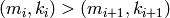
‘wall’ or ‘wall_long’: Wall’s basis. For any pair of integers
with  , let
, let
 .
The elements of Wall’s basis are monomials
.
The elements of Wall’s basis are monomials
 with
with
 , ordered left
lexicographically.
, ordered left
lexicographically.
(Note that is the reverse of the element
used in defining Arnon’s A basis.)
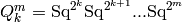
The standard way of printing elements of the Wall basis is to write
elements in terms of the . If one sets the basis to
‘wall_long’ instead of ‘wall’, then each is
expanded as a product of factors of the form
.
‘arnon_a’ or ‘arnon_a_long’: Arnon’s A basis. For any pair of
integers with , let
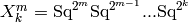 .
The elements of Arnon’s A basis are monomials
.
The elements of Arnon’s A basis are monomials
 with
with
 , ordered left
lexicographically.
, ordered left
lexicographically.
(Note that is the reverse of the element
used in defining Wall’s basis.)
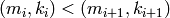
The standard way of printing elements of Arnon’s A basis is to
write elements in terms of the . If one sets the
basis to ‘arnon_a_long’ instead of ‘arnon_a’, then each
is expanded as a product of factors of the form
.
‘arnon_c’: Arnon’s C basis. The elements of Arnon’s C basis are
monomials of the form
where for each
, we have and
.
‘pst’, ‘pst_rlex’, ‘pst_llex’, ‘pst_deg’, ‘pst_revz’:
various -bases. For integers  and
and
 , the element is the Milnor basis
element
, the element is the Milnor basis
element  , with
the nonzero entry in position
, with
the nonzero entry in position  . To obtain a
-basis, for each set
. To obtain a
-basis, for each set
 of
(distinct) ‘s, one chooses an ordering and forms
the resulting monomial. The set of all such monomials then forms a
basis, and so one gets a basis by choosing an ordering on each
monomial.
of
(distinct) ‘s, one chooses an ordering and forms
the resulting monomial. The set of all such monomials then forms a
basis, and so one gets a basis by choosing an ordering on each
monomial.
The strings ‘rlex’, ‘llex’, etc., correspond to the following
orderings. These are all ‘global’ - they give a global ordering on
the ‘s, not different orderings depending on the
monomial. They order the ‘s using the pair of
integers  as follows:
‘rlex’: right lexicographic ordering
‘llex’: left lexicographic ordering
‘deg’: ordered by degree, which is the same as left
lexicographic ordering on the pair 
‘revz’: left lexicographic ordering on the pair
 , which is the reverse of the ordering used (on
elements in the same degrees as the ‘s) in Wood’s Z
basis: ‘revz’ stands for ‘reversed Z’. This is the default: ‘pst’
is the same as ‘pst_revz’.
, which is the reverse of the ordering used (on
elements in the same degrees as the ‘s) in Wood’s Z
basis: ‘revz’ stands for ‘reversed Z’. This is the default: ‘pst’
is the same as ‘pst_revz’.
‘comm’, ‘comm_rlex’, ‘comm_llex’, ‘comm_deg’, ‘comm_revz’,
or any of these with ‘_long’ appended: various commutator bases.
Let  , let
, let
![c_{i,2} = [c_{i,1}, c_{i+1,1}]](../../_images/math/455d5d0ec668f833148ec44b161751f2e8d24d31.png) , and
inductively define
, and
inductively define
![c_{i,k} = [c_{i,k-1}, c_{i+k-1,1}]](../../_images/math/c8d5ac74dd65377e83e7b0f695449291720e8b63.png) . Thus
. Thus
 is a
is a  -fold iterated commutator of the
elements , ...,
-fold iterated commutator of the
elements , ...,
 . Note that
 .
.
To obtain a commutator basis, for each set
 of
(distinct)
of
(distinct)  ‘s, one chooses an ordering and forms
the resulting monomial. The set of all such monomials then forms a
basis, and so one gets a basis by choosing an ordering on each
monomial. The strings ‘rlex’, etc., have the same meaning as for
the orderings on -bases. As with the
-bases, ‘comm_revz’ is the default: ‘comm’ means
‘comm_revz’.
‘s, one chooses an ordering and forms
the resulting monomial. The set of all such monomials then forms a
basis, and so one gets a basis by choosing an ordering on each
monomial. The strings ‘rlex’, etc., have the same meaning as for
the orderings on -bases. As with the
-bases, ‘comm_revz’ is the default: ‘comm’ means
‘comm_revz’.
The commutator bases have alternative representations, obtained by
appending ‘long’ to their names: instead of, say,
 , the representation is
  ,
indicating the commutator of
,
indicating the commutator of  and
and
 , and
, and  , which is equal to
![[[\text{Sq}^1, \text{Sq}^2], \text{Sq}^4]](../../_images/math/342a3fff0c6f39487f0eed9878e7a9a8381443cc.png) , is written as
, is written as
 .
.
EXAMPLES:
sage: steenrod_algebra_basis(7,'milnor')
(Sq(0,0,1), Sq(1,2), Sq(4,1), Sq(7))
sage: steenrod_algebra_basis(5)   # milnor basis is the default
(Sq(2,1), Sq(5))
The third (optional) argument to ‘steenrod_algebra_basis’ is the prime p:
sage: steenrod_algebra_basis(9, 'milnor', p=3)
(Q_1 P(1), Q_0 P(2))
sage: steenrod_algebra_basis(9, 'milnor', 3)
(Q_1 P(1), Q_0 P(2))
sage: steenrod_algebra_basis(17, 'milnor', 3)
(Q_2, Q_1 P(3), Q_0 P(0,1), Q_0 P(4))
Other bases:
sage: steenrod_algebra_basis(7,'admissible')
(Sq^{7}, Sq^{6} Sq^{1}, Sq^{4} Sq^{2} Sq^{1}, Sq^{5} Sq^{2})
sage: [x.basis('milnor') for x in steenrod_algebra_basis(7,'admissible')]
[Sq(7),
Sq(4,1) + Sq(7),
Sq(0,0,1) + Sq(1,2) + Sq(4,1) + Sq(7),
Sq(1,2) + Sq(7)]
sage: steenrod_algebra_basis(13,'admissible',p=3)
(beta P^{3}, P^{3} beta)
sage: steenrod_algebra_basis(5,'wall')
(Q^{2}_{2} Q^{0}_{0}, Q^{1}_{1} Q^{1}_{0})
sage: steenrod_algebra_basis(5,'wall_long')
(Sq^{4} Sq^{1}, Sq^{2} Sq^{1} Sq^{2})
sage: steenrod_algebra_basis(5,'pst-rlex')
(P^{0}_{1} P^{2}_{1}, P^{1}_{1} P^{0}_{2})
This performs crude error checking.
INPUT:
OUTPUT: None
This checks to see if the different bases have the same length, and if the change-of-basis matrices are invertible. If something goes wrong, an error message is printed.
This function checks at the prime p as the dimension goes up from 0, in which case the basis functions use the saved basis computations in lower dimensions in the computations. It also checks as the dimension goes down from the top, in which case it doesn’t have access to the saved computations. (The saved computations are deleted first: the cache _steenrod_bases is set to {} before doing the computations.)
EXAMPLES:
sage: sage.algebras.steenrod_algebra_bases.steenrod_basis_error_check(12,2)
p=2, in decreasing order of dimension, starting in dimension 12.
down to dimension  10
down to dimension  5
p=2, now in increasing order of dimension, up to dimension 12
up to dimension  0
up to dimension  5
up to dimension  10
done checking
sage: sage.algebras.steenrod_algebra_bases.steenrod_basis_error_check(30,3)
p=3, in decreasing order of dimension, starting in dimension 30.
down to dimension  30
down to dimension  25
down to dimension  20
down to dimension  15
down to dimension  10
down to dimension  5
p=3, now in increasing order of dimension, up to dimension 30
up to dimension  0
up to dimension  5
up to dimension  10
up to dimension  15
up to dimension  20
up to dimension  25
done checking
Decreasing list of degrees of the xi_i’s, starting in degree n.
INPUT:
OUTPUT:
When : decreasing list of the degrees of the
 ‘s with degree at most n.
At odd primes: decreasing list of these degrees, each divided by
 .
.
EXAMPLES:
sage: sage.algebras.steenrod_algebra_bases.xi_degrees(17)
[15, 7, 3, 1]
sage: sage.algebras.steenrod_algebra_bases.xi_degrees(17,p=3)
[13, 4, 1]
sage: sage.algebras.steenrod_algebra_bases.xi_degrees(400,p=17)
[307, 18, 1]
