Linear codes and ciphers¶

Codes¶

A linear code of length $n$ is a finite dimensional subspace of $GF(q)^n$ . Sage can compute with linear error-correcting codes to a limited extent. It basically has some wrappers to GAP and GUAVA 2.8 commands (GUAVA 2.8 does not include any of Leon’s C code which was included in previous versions of GUAVA). GUAVA 2.8 is included with Sage’s install of GAP 4.4.7 and later.

Sage can compute Hamming codes

sage: C = HammingCode(3,GF(3))
sage: C
Linear code of length 13, dimension 10 over Finite Field of size 3
sage: C.minimum_distance()
3
sage: C.gen_mat()
    [1 0 0 0 0 0 0 0 2 0 0 2 1]
    [0 1 0 0 0 0 0 0 2 0 0 2 0]
    [0 0 1 0 0 0 0 0 2 0 0 2 2]
    [0 0 0 1 0 0 0 0 2 0 0 1 0]
    [0 0 0 0 1 0 0 0 2 0 0 1 2]
    [0 0 0 0 0 1 0 0 2 0 0 1 1]
    [0 0 0 0 0 0 1 0 2 0 0 0 2]
    [0 0 0 0 0 0 0 1 2 0 0 0 1]
    [0 0 0 0 0 0 0 0 0 1 0 2 2]
    [0 0 0 0 0 0 0 0 0 0 1 2 1]

the four Golay codes

sage: C = ExtendedTernaryGolayCode()
sage: C
Linear code of length 12, dimension 6 over Finite Field of size 3
sage: C.minimum_distance()
6
sage: C.gen_mat()
[1 0 0 0 0 0 2 0 1 2 1 2]
[0 1 0 0 0 0 1 2 2 2 1 0]
[0 0 1 0 0 0 1 1 1 0 1 1]
[0 0 0 1 0 0 1 1 0 2 2 2]
[0 0 0 0 1 0 2 1 2 2 0 1]
[0 0 0 0 0 1 0 2 1 2 2 1]

as well as binary Reed-Muller codes, quadratic residue codes, quasi-quadratic residue codes, “random” linear codes, and a code generated by a matrix of full rank (using, as usual, the rows as the basis).

For a given code, $C$ , Sage can return a generator matrix, a check matrix, and the dual code:

sage: C = HammingCode(3,GF(2))
sage: Cperp = C.dual_code()
sage: C; Cperp
Linear code of length 7, dimension 4 over Finite Field of size 2
Linear code of length 7, dimension 3 over Finite Field of size 2
sage: C.gen_mat()
   [1 0 0 1 0 1 0]
   [0 1 0 1 0 1 1]
   [0 0 1 1 0 0 1]
   [0 0 0 0 1 1 1]
sage: C.check_mat()
   [1 0 0 1 1 0 1]
   [0 1 0 1 0 1 1]
   [0 0 1 1 1 1 0]
sage: C.dual_code()
Linear code of length 7, dimension 3 over Finite Field of size 2
sage: C = HammingCode(3,GF(4,'a'))
sage: C.dual_code()
Linear code of length 21, dimension 3 over Finite Field in a of size 2^2

For $C$ and a vector $v\in GF(q)^n$ , Sage can try to decode $v$ (i.e., find the codeword $c\in C$ closest to $v$ in the Hamming metric) using syndrome decoding. As of yet, no special decoding methods have been implemented.

sage: C = HammingCode(3,GF(2))
sage: MS = MatrixSpace(GF(2),1,7)
sage: F = GF(2); a = F.gen()
sage: v1 = [a,a,F(0),a,a,F(0),a]
sage: C.decode(v1)
(1, 0, 0, 1, 1, 0, 1)
sage: v2 = matrix([[a,a,F(0),a,a,F(0),a]])
sage: C.decode(v2)
(1, 0, 0, 1, 1, 0, 1)
sage: v3 = vector([a,a,F(0),a,a,F(0),a])
sage: c = C.decode(v3); c
(1, 0, 0, 1, 1, 0, 1)

To plot the (histogram of) the weight distribution of a code, one can use the matplotlib package included with Sage:

sage: C = HammingCode(4,GF(2))
sage: C
 Linear code of length 15, dimension 11 over Finite Field of size 2
sage: w = C.weight_distribution(); w
 [1, 0, 0, 35, 105, 168, 280, 435, 435, 280, 168, 105, 35, 0, 0, 1]
sage: J = range(len(w))
sage: W = IndexedSequence([ZZ(w[i]) for i in J],J)
sage: P = W.plot_histogram()

Now type show(P) to view this.

There are several coding theory functions we are skipping entirely. Please see the reference manual or the file coding/linear_codes.py for examples.

Sage can also compute algebraic-geometric codes, called AG codes, via the Singular interface § sec:agcodes. One may also use the AG codes implemented in GUAVA via the Sage interface to GAP gap_console(). See the GUAVA manual for more details. {GUAVA}

Ciphers¶

LFSRs¶

A special type of stream cipher is implemented in Sage, namely, a linear feedback shift register (LFSR) sequence defined over a finite field. Stream ciphers have been used for a long time as a source of pseudo-random number generators. {linear feedback shift register}

S. Golomb {G} gives a list of three statistical properties a sequence of numbers ${\bf a}=\{a_n\}_{n=1}^\infty$ , $a_n\in \{0,1\}$ , should display to be considered “random”. Define the autocorrelation of ${\bf a}$ to be

$C(k)=C(k,{\bf a})=\lim_{N\rightarrow \infty} \frac{1}{N}\sum_{n=1}^N (-1)^{a_n+a_{n+k}}.$

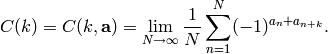
In the case where $a$ is periodic with period $P$ then this reduces to

Assume $a$ is periodic with period $P$ .

balance: $|\sum_{n=1}^P(-1)^{a_n}|\leq 1$ .
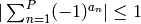low autocorrelation:

$C(k)= \left\{ \begin{array}{cc} 1,& k=0,\\ \epsilon, & k\not= 0. \end{array} \right.$

(For sequences satisfying these first two properties, it is known that $\epsilon=-1/P$ must hold.)
proportional runs property: In each period, half the runs have length $1$ , one-fourth have length $2$ , etc. Moveover, there are as many runs of $1$ ‘s as there are of $0$ ‘s.

A sequence satisfying these properties will be called pseudo-random. {pseudo-random}

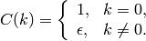
A general feedback shift register is a map $f:{\bf F}_q^d\rightarrow {\bf F}_q^d$ of the form

$\begin{array}{c} f(x_0,...,x_{n-1})=(x_1,x_2,...,x_n),\\ x_n=C(x_0,...,x_{n-1}), \end{array}$

where $C:{\bf F}_q^d\rightarrow {\bf F}_q$ is a given function. When $C$ is of the form

..math:: C(x_0,...,x_{n-1})=c_0x_0+...+c_{n-1}x_{n-1},

for some given constants $c_i\in {\bf F}_q$ , the map is called a linear feedback shift register (LFSR). The sequence of coefficients $c_i$ is called the key and the polynomial

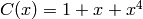
is sometimes called the connection polynomial.

Example: Over $GF(2)$ , if $[c_0,c_1,c_2,c_3]=[1,0,0,1]$ then $C(x) = 1 + x + x^4$ ,

The LFSR sequence is then

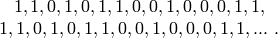
$\begin{array}{c} 1, 1, 0, 1, 0, 1, 1, 0, 0, 1, 0, 0, 0, 1, 1, \\ 1, 1, 0, 1, 0, 1, 1, 0, 0, 1, 0, 0, 0, 1, 1, ...\ . \end{array}$

The sequence of $0,1$ ‘s is periodic with period $P=2^4-1=15$ and satisfies Golomb’s three randomness conditions. However, this sequence of period 15 can be “cracked” (i.e., a procedure to reproduce $g(x)$ ) by knowing only 8 terms! This is the function of the Berlekamp-Massey algorithm {M}, implemented as lfsr_connection_polynomial (which produces the reverse of berlekamp_massey).

sage: F = GF(2)
sage: o = F(0)
sage: l = F(1)
sage: key = [l,o,o,l]; fill = [l,l,o,l]; n = 20
sage: s = lfsr_sequence(key,fill,n); s
[1, 1, 0, 1, 0, 1, 1, 0, 0, 1, 0, 0, 0, 1, 1, 1, 1, 0, 1, 0]
sage: lfsr_autocorrelation(s,15,7)
4/15
sage: lfsr_autocorrelation(s,15,0)
8/15
sage: lfsr_connection_polynomial(s)
x^4 + x + 1
sage: berlekamp_massey(s)
x^4 + x^3 + 1

Classical ciphers¶

has a type for cryptosystems (created by David Kohel, who also wrote the examples below), implementing classical cryptosystems. The general interface is as follows:

sage: S = AlphabeticStrings()
sage: S
Free alphabetic string monoid on A-Z
sage: E = SubstitutionCryptosystem(S)
sage: E
Substitution cryptosystem on Free alphabetic string monoid on A-Z
sage: K = S([ 25-i for i in range(26) ])
sage: e = E(K)
sage: m = S("THECATINTHEHAT")
sage: e(m)
GSVXZGRMGSVSZG

Here’s another example:

sage: S = AlphabeticStrings()
sage: E = TranspositionCryptosystem(S,15);
sage: m = S("THECATANDTHEHAT")
sage: G = E.key_space()
sage: G
Symmetric group of order 15! as a permutation group
sage: g = G([ 3, 2, 1, 6, 5, 4, 9, 8, 7, 12, 11, 10, 15, 14, 13 ])
sage: e = E(g)
sage: e(m)
EHTTACDNAEHTTAH

The idea is that a cryptosystem is a map $E: KS \to \text{Hom}_\text{Set}(MS,CS)$ where $KS$ , $MS$ , and $CS$ are the key space, plaintext (or message) space, and ciphertext space, respectively. $E$ is presumed to be injective, so e.key() returns the pre-image key.

Linear codes and ciphers¶

Codes¶

Ciphers¶

LFSRs¶

Classical ciphers¶

Table Of Contents

Previous topic

Next topic

This Page

Navigation

Linear codes and ciphers¶

Codes¶

Ciphers¶

LFSRs¶

Classical ciphers¶

Table Of Contents

Previous topic

Next topic

This Page

Quick search

Navigation