Miscellaneous arithmetic functions¶

sage.rings.arith.CRT(a, b, m=None, n=None)¶

Returns a solution to a Chinese Remainder Theorem problem.

INPUT:

a, b - two residues (elements of some ring for which extended gcd is available), or two lists, one of residues and one of moduli.
m, n - (default: None) two moduli, or None.

OUTPUT:

If m, n are not None, returns a solution $x$ to the simultaneous congruences $x\equiv a \bmod m$ and $x\equiv b \bmod n$ , if one exists. By the Chinese Remainder Theorem, a solution to the simultaneous congruences exists if and only if $a\equiv b\pmod{\gcd(m,n)}$ . The solution $x$ is only well-defined modulo $\text{lcm}(m,n)$ .

If a and b are lists, returns a simultaneous solution to the congruences $x\equiv a_i\pmod{b_i}$ , if one exists.

See also

crt()

EXAMPLES:

sage: CRT_list([2,3,2], [3,5,7])
23
sage: x = polygen(QQ)
sage: c = CRT_list([3], [x]); c
3
sage: c.parent()
Univariate Polynomial Ring in x over Rational Field

The arguments must be lists:

sage: CRT_list([1,2,3],"not a list")
...
ValueError: Arguments to CRT_list should be lists
sage: CRT_list("not a list",[2,3])  
...
ValueError: Arguments to CRT_list should be lists

The list of moduli must have the same length as the list of elements:

sage: CRT_list([1,2,3],[2,3,5])       
23
sage: CRT_list([1,2,3],[2,3])    
...
ValueError: Arguments to CRT_list should be lists of the same length
sage: CRT_list([1,2,3],[2,3,5,7])
...
ValueError: Arguments to CRT_list should be lists of the same length

sage.rings.arith.CRT_vectors(X, moduli)¶

Vector form of the Chinese Remainder Theorem: given a list of integer vectors $v_i$ and a list of coprime moduli $m_i$ , find a vector $w$ such that $w = v_i \pmod m_i$ for all $i$ . This is more efficient than applying CRT() to each entry.

INPUT:

X - list or tuple, consisting of lists/tuples/vectors/etc of integers of the same length
moduli - list of len(X) moduli

OUTPUT:

list - application of CRT componentwise.

EXAMPLES:

sage: CRT_vectors([[3,5,7],[3,5,11]], [2,3])
[3, 5, 5]

sage: CRT_vectors([vector(ZZ, [2,3,1]), Sequence([1,7,8],ZZ)], [8,9])
[10, 43, 17]

class sage.rings.arith.Euler_Phi¶

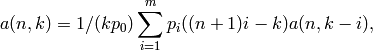
Return the value of the Euler phi function on the integer n. We defined this to be the number of positive integers <= n that are relatively prime to n. Thus if n<=0 then euler_phi(n) is defined and equals 0.

INPUT:

n - an integer

EXAMPLES:

sage: euler_phi(1)
1
sage: euler_phi(2)
1
sage: euler_phi(3)
2
sage: euler_phi(12)
4
sage: euler_phi(37)
36

Notice that euler_phi is defined to be 0 on negative numbers and 0.

sage: euler_phi(-1)  
0
sage: euler_phi(0)
0
sage: type(euler_phi(0))
<type 'sage.rings.integer.Integer'>

We verify directly that the phi function is correct for 21.

sage: euler_phi(21)
12
sage: [i for i in range(21) if gcd(21,i) == 1]
[1, 2, 4, 5, 8, 10, 11, 13, 16, 17, 19, 20]

The length of the list of integers ‘i’ in range(n) such that the gcd(i,n) == 1 equals euler_phi(n).

sage: len([i for i in range(21) if gcd(21,i) == 1]) == euler_phi(21)
True

The phi function also has a special plotting method.

sage: P = plot(euler_phi, -3, 71)

AUTHORS:

William Stein
Alex Clemesha (2006-01-10): some examples

plot(xmin=1, xmax=50, pointsize=30, rgbcolor=(0, 0, 1), join=True, **kwds)¶

Plot the Euler phi function.

INPUT:

xmin - default: 1
xmax - default: 50
pointsize - default: 30
rgbcolor - default: (0,0,1)
join - default: True; whether to join the points.
**kwds - passed on

EXAMPLES:

sage: p = Euler_Phi().plot()
sage: p.ymax()
46.0

sage.rings.arith.GCD(a, b=None, **kwargs)¶

The greatest common divisor of a and b, or if a is a list and b is omitted the greatest common divisor of all elements of a.

INPUT:

a,b - two elements of a ring with gcd or
a - a list or tuple of elements of a ring with gcd

Additional keyword arguments are passed to the respectively called methods.

EXAMPLES:

sage: GCD(97,100)
1
sage: GCD(97*10^15, 19^20*97^2)
97
sage: GCD(2/3, 4/3)
1
sage: GCD([2,4,6,8])
2
sage: GCD(srange(0,10000,10))  # fast  !!
10

Note that to take the gcd of $n$ elements for $n \not= 2$ you must put the elements into a list by enclosing them in [..]. Before #4988 the following wrongly returned 3 since the third parameter was just ignored:

sage: gcd(3,6,2)
...
TypeError: gcd() takes at most 2 arguments (3 given)
sage: gcd([3,6,2])
1

Similarly, giving just one element (which is not a list) gives an error:

sage: gcd(3)
...
TypeError: 'sage.rings.integer.Integer' object is not iterable

By convention, the gcd of the empty list is (the integer) 0:

sage: gcd([])
0
sage: type(gcd([]))
<type 'sage.rings.integer.Integer'>

sage.rings.arith.LCM(a, b=None)¶

The least common multiple of a and b, or if a is a list and b is omitted the least common multiple of all elements of a.

Note that LCM is an alias for lcm.

INPUT:

a,b - two elements of a ring with lcm or
a - a list or tuple of elements of a ring with lcm

EXAMPLES:

sage: lcm(97,100)
9700
sage: LCM(97,100)
9700
sage: LCM(0,2)
0
sage: LCM(-3,-5)
15
sage: LCM([1,2,3,4,5])
60
sage: v = LCM(range(1,10000))   # *very* fast!
sage: len(str(v))
4349

class sage.rings.arith.Moebius¶

Returns the value of the Moebius function of abs(n), where n is an integer.

DEFINITION: $\mu(n)$ is 0 if $n$ is not square free, and otherwise equals $(-1)^r$ , where $n$ has $r$ distinct prime factors.

For simplicity, if $n=0$ we define $\mu(n) = 0$ .

IMPLEMENTATION: Factors or - for integers - uses the PARI C library.

INPUT:

n - anything that can be factored.

OUTPUT: 0, 1, or -1

EXAMPLES:

sage: moebius(-5)
-1
sage: moebius(9)
0
sage: moebius(12)
0
sage: moebius(-35)
1
sage: moebius(-1)
1
sage: moebius(7)
-1

sage: moebius(0)   # potentially nonstandard!
0

The moebius function even makes sense for non-integer inputs.

sage: x = GF(7)['x'].0
sage: moebius(x+2)
-1

plot(xmin=0, xmax=50, pointsize=30, rgbcolor=(0, 0, 1), join=True, **kwds)¶

Plot the Moebius function.

INPUT:

xmin - default: 0
xmax - default: 50
pointsize - default: 30
rgbcolor - default: (0,0,1)
join - default: True; whether to join the points (very helpful in seeing their order).
**kwds - passed on

EXAMPLES:

sage: p = Moebius().plot()
sage: p.ymax()
1.0

range(start, stop=None, step=None)¶

Return the Moebius function evaluated at the given range of values, i.e., the image of the list range(start, stop, step) under the Mobius function.

This is much faster than directly computing all these values with a list comprehension.

EXAMPLES:

sage: v = moebius.range(-10,10); v
[1, 0, 0, -1, 1, -1, 0, -1, -1, 1, 0, 1, -1, -1, 0, -1, 1, -1, 0, 0]
sage: v == [moebius(n) for n in range(-10,10)]
True
sage: v = moebius.range(-1000, 2000, 4)
sage: v == [moebius(n) for n in range(-1000,2000, 4)]
True

class sage.rings.arith.Sigma¶

Return the sum of the k-th powers of the divisors of n.

INPUT:

n - integer
k - integer (default: 1)

OUTPUT: integer

EXAMPLES:

sage: sigma(5)
6
sage: sigma(5,2)
26

The sigma function also has a special plotting method.

sage: P = plot(sigma, 1, 100)

This method also works with k-th powers.

sage: P = plot(sigma, 1, 100, k=2)

AUTHORS:

William Stein: original implementation
Craig Citro (2007-06-01): rewrote for huge speedup

TESTS:

sage: sigma(100,4)
106811523
sage: sigma(factorial(100),3).mod(144169)
3672
sage: sigma(factorial(150),12).mod(691)
176
sage: RR(sigma(factorial(133),20))
2.80414775675747e4523
sage: sigma(factorial(100),0)
39001250856960000
sage: sigma(factorial(41),1)
229199532273029988767733858700732906511758707916800

plot(xmin=1, xmax=50, k=1, pointsize=30, rgbcolor=(0, 0, 1), join=True, **kwds)¶

Plot the sigma (sum of k-th powers of divisors) function.

INPUT:

xmin - default: 1
xmax - default: 50
k - default: 1
pointsize - default: 30
rgbcolor - default: (0,0,1)
join - default: True; whether to join the points.
**kwds - passed on

EXAMPLES:

sage: p = Sigma().plot()
sage: p.ymax()
124.0

sage.rings.arith.XGCD(a, b)¶

Return a triple (g,s,t) such that $g = s\cdot a+t\cdot b = \gcd(a,b)$ .

Note

One exception is if $a$ and $b$ are not in a PID, e.g., they are both polynomials over the integers, then this function can’t in general return (g,s,t) as above, since they need not exist. Instead, over the integers, we first multiply $g$ by a divisor of the resultant of $a/g$ and $b/g$ , up to sign.

INPUT:

a, b - integers or univariate polynomials (or any type with an xgcd method).

OUTPUT:

g, s, t - such that $g = s\cdot a + t\cdot b$

Note

There is no guarantee that the returned cofactors (s and t) are minimal. In the integer case, see sage.rings.integer.Integer._xgcd() for minimal cofactors.

EXAMPLES:

sage: xgcd(56, 44)
(4, 4, -5)
sage: 4*56 + (-5)*44
4
sage: g, a, b = xgcd(5/1, 7/1); g, a, b
(1, 3, -2)
sage: a*(5/1) + b*(7/1) == g
True
sage: x = polygen(QQ)
sage: xgcd(x^3 - 1, x^2 - 1)
(x - 1, 1, -x)
sage: K.<g> = NumberField(x^2-3)
sage: R.<a,b> = K[]
sage: S.<y> = R.fraction_field()[]
sage: xgcd(y^2, a*y+b)
(1, a^2/b^2, ((-a)/b^2)*y + 1/b)
sage: xgcd((b+g)*y^2, (a+g)*y+b)
(1, (a^2 + (2*g)*a + 3)/(b^3 + (g)*b^2), ((-a + (-g))/b^2)*y + 1/b)

We compute an xgcd over the integers, where the linear combination is not the gcd but the resultant:

sage: R.<x> = ZZ[]
sage: gcd(2*x*(x-1), x^2)
x
sage: xgcd(2*x*(x-1), x^2)
(2*x, -1, 2)
sage: (2*(x-1)).resultant(x)
2

sage.rings.arith.algdep(z, degree, known_bits=None, use_bits=None, known_digits=None, use_digits=None, height_bound=None, proof=False)¶

Returns a polynomial of degree at most $degree$ which is approximately satisfied by the number $z$ . Note that the returned polynomial need not be irreducible, and indeed usually won’t be if $z$ is a good approximation to an algebraic number of degree less than $degree$ .

You can specify the number of known bits or digits with known_bits=k or known_digits=k; Pari is then told to compute the result using $0.8k$ of these bits/digits. (The Pari documentation recommends using a factor between .6 and .9, but internally defaults to .8.) Or, you can specify the precision to use directly with use_bits=k or use_digits=k. If none of these are specified, then the precision is taken from the input value.

A height bound may specified to indicate the maximum coefficient size of the returned polynomial; if a sufficiently small polyomial is not found then None wil be returned. If proof=True then the result is returned only if it can be proved correct (i.e. the only possible minimal polynomial satisfying the height bound, or no such polynomial exists). Otherwise a ValueError is raised indicating that higher precision is required.

ALGORITHM: Uses LLL for real/complex inputs, PARI C-library algdep command otherwise.

Note that algebraic_dependency is a synonym for algdep.

INPUT:

z - real, complex, or $p$ -adic number
degree - an integer
height_bound - an integer (default None) specifying the maximum

coefficient size for the returned polynomial
proof - a boolean (default False), requres height_bound to be set

EXAMPLES:

sage: algdep(1.888888888888888, 1)
9*x - 17
sage: algdep(0.12121212121212,1)
33*x - 4
sage: algdep(sqrt(2),2)
x^2 - 2

This example involves a complex number.

sage: z = (1/2)*(1 + RDF(sqrt(3)) *CC.0); z
0.500000000000000 + 0.866025403784439*I
sage: p = algdep(z, 6); p
x^3 + 1
sage: p.factor()
(x + 1) * (x^2 - x + 1)
sage: z^2 - z + 1
0

This example involves a $p$ -adic number.

sage: K = Qp(3, print_mode = 'series')
sage: a = K(7/19); a
1 + 2*3 + 3^2 + 3^3 + 2*3^4 + 2*3^5 + 3^8 + 2*3^9 + 3^11 + 3^12 + 2*3^15 + 2*3^16 + 3^17 + 2*3^19 + O(3^20)
sage: algdep(a, 1)
19*x - 7

These examples show the importance of proper precision control. We compute a 200-bit approximation to sqrt(2) which is wrong in the 33’rd bit.

sage: z = sqrt(RealField(200)(2)) + (1/2)^33
sage: p = algdep(z, 4); p
227004321085*x^4 - 216947902586*x^3 - 99411220986*x^2 + 82234881648*x - 211871195088
sage: factor(p)
227004321085*x^4 - 216947902586*x^3 - 99411220986*x^2 + 82234881648*x - 211871195088
sage: algdep(z, 4, known_bits=32)
x^2 - 2
sage: algdep(z, 4, known_digits=10)
x^2 - 2
sage: algdep(z, 4, use_bits=25)
x^2 - 2
sage: algdep(z, 4, use_digits=8)
x^2 - 2

Using the height_bound and proof parameters, we can see that $pi$ is not the root of an integer polynomial of degree at most 5 and coefficients bounded above by 10.

sage: algdep(pi.n(), 5, height_bound=10, proof=True) is None
True

For stronger results, we need more precicion.

sage: algdep(pi.n(), 5, height_bound=100, proof=True) is None
...
ValueError: insufficient precision for non-existence proof
sage: algdep(pi.n(200), 5, height_bound=100, proof=True) is None
True

sage: algdep(pi.n(), 10, height_bound=10, proof=True) is None
...
ValueError: insufficient precision for non-existence proof
sage: algdep(pi.n(200), 10, height_bound=10, proof=True) is None
True

We can also use proof=True to get positive results.

sage: a = sqrt(2) + sqrt(3) + sqrt(5)
sage: algdep(a.n(), 8, height_bound=1000, proof=True)
...
ValueError: insufficient precision for uniqueness proof
sage: f = algdep(a.n(1000), 8, height_bound=1000, proof=True); f
x^8 - 40*x^6 + 352*x^4 - 960*x^2 + 576
sage: f(a).expand()
0

sage.rings.arith.algebraic_dependency(z, degree, known_bits=None, use_bits=None, known_digits=None, use_digits=None, height_bound=None, proof=False)¶

Returns a polynomial of degree at most $degree$ which is approximately satisfied by the number $z$ . Note that the returned polynomial need not be irreducible, and indeed usually won’t be if $z$ is a good approximation to an algebraic number of degree less than $degree$ .

You can specify the number of known bits or digits with known_bits=k or known_digits=k; Pari is then told to compute the result using $0.8k$ of these bits/digits. (The Pari documentation recommends using a factor between .6 and .9, but internally defaults to .8.) Or, you can specify the precision to use directly with use_bits=k or use_digits=k. If none of these are specified, then the precision is taken from the input value.

A height bound may specified to indicate the maximum coefficient size of the returned polynomial; if a sufficiently small polyomial is not found then None wil be returned. If proof=True then the result is returned only if it can be proved correct (i.e. the only possible minimal polynomial satisfying the height bound, or no such polynomial exists). Otherwise a ValueError is raised indicating that higher precision is required.

ALGORITHM: Uses LLL for real/complex inputs, PARI C-library algdep command otherwise.

Note that algebraic_dependency is a synonym for algdep.

INPUT:

z - real, complex, or $p$ -adic number
degree - an integer
height_bound - an integer (default None) specifying the maximum

coefficient size for the returned polynomial
proof - a boolean (default False), requres height_bound to be set

EXAMPLES:

sage: algdep(1.888888888888888, 1)
9*x - 17
sage: algdep(0.12121212121212,1)
33*x - 4
sage: algdep(sqrt(2),2)
x^2 - 2

This example involves a complex number.

sage: z = (1/2)*(1 + RDF(sqrt(3)) *CC.0); z
0.500000000000000 + 0.866025403784439*I
sage: p = algdep(z, 6); p
x^3 + 1
sage: p.factor()
(x + 1) * (x^2 - x + 1)
sage: z^2 - z + 1
0

This example involves a $p$ -adic number.

sage: K = Qp(3, print_mode = 'series')
sage: a = K(7/19); a
1 + 2*3 + 3^2 + 3^3 + 2*3^4 + 2*3^5 + 3^8 + 2*3^9 + 3^11 + 3^12 + 2*3^15 + 2*3^16 + 3^17 + 2*3^19 + O(3^20)
sage: algdep(a, 1)
19*x - 7

These examples show the importance of proper precision control. We compute a 200-bit approximation to sqrt(2) which is wrong in the 33’rd bit.

sage: z = sqrt(RealField(200)(2)) + (1/2)^33
sage: p = algdep(z, 4); p
227004321085*x^4 - 216947902586*x^3 - 99411220986*x^2 + 82234881648*x - 211871195088
sage: factor(p)
227004321085*x^4 - 216947902586*x^3 - 99411220986*x^2 + 82234881648*x - 211871195088
sage: algdep(z, 4, known_bits=32)
x^2 - 2
sage: algdep(z, 4, known_digits=10)
x^2 - 2
sage: algdep(z, 4, use_bits=25)
x^2 - 2
sage: algdep(z, 4, use_digits=8)
x^2 - 2

Using the height_bound and proof parameters, we can see that $pi$ is not the root of an integer polynomial of degree at most 5 and coefficients bounded above by 10.

sage: algdep(pi.n(), 5, height_bound=10, proof=True) is None
True

For stronger results, we need more precicion.

sage: algdep(pi.n(), 5, height_bound=100, proof=True) is None
...
ValueError: insufficient precision for non-existence proof
sage: algdep(pi.n(200), 5, height_bound=100, proof=True) is None
True

sage: algdep(pi.n(), 10, height_bound=10, proof=True) is None
...
ValueError: insufficient precision for non-existence proof
sage: algdep(pi.n(200), 10, height_bound=10, proof=True) is None
True

We can also use proof=True to get positive results.

sage: a = sqrt(2) + sqrt(3) + sqrt(5)
sage: algdep(a.n(), 8, height_bound=1000, proof=True)
...
ValueError: insufficient precision for uniqueness proof
sage: f = algdep(a.n(1000), 8, height_bound=1000, proof=True); f
x^8 - 40*x^6 + 352*x^4 - 960*x^2 + 576
sage: f(a).expand()
0

sage.rings.arith.bernoulli(n, algorithm='default', num_threads=1)¶

Return the n-th Bernoulli number, as a rational number.

INPUT:

n - an integer
algorithm:
- 'default' - (default) use ‘pari’ for n <= 30000, and ‘bernmm’ for n > 30000 (this is just a heuristic, and not guaranteed to be optimal on all hardware)
- 'pari' - use the PARI C library
- 'gap' - use GAP
- 'gp' - use PARI/GP interpreter
- 'magma' - use MAGMA (optional)
- 'bernmm' - use bernmm package (a multimodular algorithm)
num_threads - positive integer, number of threads to use (only used for bernmm algorithm)

EXAMPLES:

sage: bernoulli(12)
-691/2730
sage: bernoulli(50)
495057205241079648212477525/66

We demonstrate each of the alternative algorithms:

sage: bernoulli(12, algorithm='gap')    
-691/2730
sage: bernoulli(12, algorithm='gp')
-691/2730
sage: bernoulli(12, algorithm='magma')           # optional - magma
-691/2730
sage: bernoulli(12, algorithm='pari')    
-691/2730
sage: bernoulli(12, algorithm='bernmm')
-691/2730
sage: bernoulli(12, algorithm='bernmm', num_threads=4)
-691/2730

TESTS:

sage: algs = ['gap','gp','pari','bernmm']
sage: test_list = [ZZ.random_element(2, 2255) for _ in range(500)]
sage: vals = [[bernoulli(i,algorithm = j) for j in algs] for i in test_list] #long time (19s)
sage: union([len(union(x))==1 for x in vals]) #long time (depends on previous line)
[True]
sage: algs = ['gp','pari','bernmm']
sage: test_list = [ZZ.random_element(2256, 5000) for _ in range(500)]
sage: vals = [[bernoulli(i,algorithm = j) for j in algs] for i in test_list] #long time (21s)
sage: union([len(union(x))==1 for x in vals]) #long time (depends on previous line)
[True]

AUTHOR:

David Joyner and William Stein

sage.rings.arith.binomial(x, m)¶

Return the binomial coefficient

$\binom{x}{m} = x (x-1) \cdots (x-m+1) / m!$

which is defined for $m \in \ZZ$ and any $x$ . We extend this definition to include cases when $x-m$ is an integer but $m$ is not by

$\binom{x}{m}= \binom{x}{x-m}$

If $m < 0$ , return $0$ .

INPUT:

x, m - numbers or symbolic expressions. Either m or x-m must be an integer.

OUTPUT: number or symbolic expression (if input is symbolic)

EXAMPLES:

sage: binomial(5,2)
10
sage: binomial(2,0)
1
sage: binomial(1/2, 0)
1
sage: binomial(3,-1)
0
sage: binomial(20,10)
184756
sage: binomial(-2, 5)
-6
sage: binomial(RealField()('2.5'), 2)
1.87500000000000
sage: n=var('n'); binomial(n,2)
1/2*(n - 1)*n
sage: n=var('n'); binomial(n,n)
1
sage: n=var('n'); binomial(n,n-1)
n
sage: binomial(2^100, 2^100)
1

sage: k, i = var('k,i')
sage: binomial(k,i)
binomial(k, i)

TESTS:

We test that certain binomials are very fast (this should be instant) – see trac 3309:

sage: a = binomial(RR(1140000.78), 42000000)

We test conversion of arguments to Integers – see trac 6870:

sage: binomial(1/2,1/1)
1/2
sage: binomial(10^20+1/1,10^20)
100000000000000000001
sage: binomial(SR(10**7),10**7) 
1
sage: binomial(3/2,SR(1/1))
3/2

Some floating point cases – see trac 7562:

sage: binomial(1.,3) 
0.000000000000000
sage: binomial(-2.,3)
-4.00000000000000

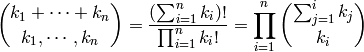
sage.rings.arith.binomial_coefficients(n)¶

Return a dictionary containing pairs $\{(k_1,k_2) : C_{k,n}\}$ where $C_{k_n}$ are binomial coefficients and $n = k_1 + k_2$ .

INPUT:

n - an integer

OUTPUT: dict

EXAMPLES:

sage: sorted(binomial_coefficients(3).items())
[((0, 3), 1), ((1, 2), 3), ((2, 1), 3), ((3, 0), 1)]

Notice the coefficients above are the same as below:

sage: R.<x,y> = QQ[]
sage: (x+y)^3
x^3 + 3*x^2*y + 3*x*y^2 + y^3

AUTHORS:

Fredrik Johansson

sage.rings.arith.continuant(v, n=None)¶

Function returns the continuant of the sequence $v$ (list or tuple).

Definition: see Graham, Knuth and Patashnik, Concrete Mathematics, section 6.7: Continuants. The continuant is defined by

$K_0() = 1$
$K_1(x_1) = x_1$
$K_n(x_1, \cdots, x_n) = K_{n-1}(x_n, \cdots x_{n-1})x_n + K_{n-2}(x_1, \cdots, x_{n-2})$

If n = None or n > len(v) the default n = len(v) is used.

INPUT:

v - list or tuple of elements of a ring
n - optional integer

OUTPUT: element of ring (integer, polynomial, etcetera).

EXAMPLES:

sage: continuant([1,2,3])
10
sage: p = continuant([2, 1, 2, 1, 1, 4, 1, 1, 6, 1, 1, 8, 1, 1, 10])
sage: q = continuant([1, 2, 1, 1, 4, 1, 1, 6, 1, 1, 8, 1, 1, 10])
sage: p/q
517656/190435
sage: convergent([2, 1, 2, 1, 1, 4, 1, 1, 6, 1, 1, 8, 1, 1, 10],14)
517656/190435
sage: x = PolynomialRing(RationalField(),'x',5).gens()
sage: continuant(x)
x0*x1*x2*x3*x4 + x0*x1*x2 + x0*x1*x4 + x0*x3*x4 + x2*x3*x4 + x0 + x2 + x4
sage: continuant(x, 3)
x0*x1*x2 + x0 + x2
sage: continuant(x,2)
x0*x1 + 1

We verify the identity

$K_n(z,z,\cdots,z) = \sum_{k=0}^n \binom{n-k}{k} z^{n-2k}$

for $n = 6$ using polynomial arithmetic:

sage: z = QQ['z'].0
sage: continuant((z,z,z,z,z,z,z,z,z,z,z,z,z,z,z),6)
z^6 + 5*z^4 + 6*z^2 + 1

sage: continuant(9)
...
TypeError: object of type 'sage.rings.integer.Integer' has no len()

AUTHORS:

Jaap Spies (2007-02-06)

sage.rings.arith.continued_fraction_list(x, partial_convergents=False, bits=None)¶

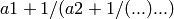
Returns the continued fraction of x as a list.

Note

This may be slow for real number input, since it’s implemented in pure Python. For rational number input the PARI C library is used.

EXAMPLES:

sage: continued_fraction_list(45/17)
[2, 1, 1, 1, 5]
sage: continued_fraction_list(e, bits=20)
[2, 1, 2, 1, 1, 4, 1, 1, 6]
sage: continued_fraction_list(e, bits=30)
[2, 1, 2, 1, 1, 4, 1, 1, 6, 1, 1, 8, 1, 1]        
sage: continued_fraction_list(sqrt(2))
[1, 2, 2, 2, 2, 2, 2, 2, 2, 2, 2, 2, 2, 2, 2, 2, 2, 2, 2, 2, 2, 1, 1]
sage: continued_fraction_list(sqrt(4/19))
[0, 2, 5, 1, 1, 2, 1, 16, 1, 2, 1, 1, 5, 4, 5, 1, 1, 2, 1, 15, 2]
sage: continued_fraction_list(RR(pi), partial_convergents=True)
([3, 7, 15, 1, 292, 1, 1, 1, 2, 1, 3, 1, 14, 3],
 [(3, 1),
  (22, 7),
  (333, 106),
  (355, 113),
  (103993, 33102),
  (104348, 33215),
  (208341, 66317),
  (312689, 99532),
  (833719, 265381),
  (1146408, 364913),
  (4272943, 1360120),
  (5419351, 1725033),
  (80143857, 25510582),
  (245850922, 78256779)])
sage: continued_fraction_list(e)
[2, 1, 2, 1, 1, 4, 1, 1, 6, 1, 1, 8, 1, 1, 10, 1, 1, 12, 1, 1, 11]
sage: continued_fraction_list(RR(e))
[2, 1, 2, 1, 1, 4, 1, 1, 6, 1, 1, 8, 1, 1, 10, 1, 1, 12, 1, 1, 11]
sage: continued_fraction_list(RealField(200)(e))
[2, 1, 2, 1, 1, 4, 1, 1, 6, 1, 1, 8, 1, 1, 10, 1, 1, 12, 1, 1, 14, 1, 1, 16, 1, 1, 18, 1, 1, 20, 1, 1, 22, 1, 1, 24, 1, 1, 26, 1, 1, 28, 1, 1, 30, 1, 1, 32, 1, 1, 34, 1, 1, 36, 1, 1, 38, 1, 1]

sage.rings.arith.convergent(v, n)¶

Return the n-th continued fraction convergent of the continued fraction defined by the sequence of integers v. We assume $n \geq 0$ .

INPUT:

v - list of integers
n - integer

OUTPUT: a rational number

If the continued fraction integers are

$v = [a_0, a_1, a_2, \ldots, a_k]$

then convergent(v,2) is the rational number

$a_0 + 1/a_1$

and convergent(v,k) is the rational number

$a1 + 1/(a2+1/(...) ... )$

represented by the continued fraction.

EXAMPLES:

sage: convergent([2, 1, 2, 1, 1, 4, 1, 1], 7)
193/71

sage.rings.arith.convergents(v)¶

Return all the partial convergents of a continued fraction defined by the sequence of integers v.

If v is not a list, compute the continued fraction of v and return its convergents (this is potentially much faster than calling continued_fraction first, since continued fractions are implemented using PARI and there is overhead moving the answer back from PARI).

INPUT:

v - list of integers or a rational number

OUTPUT:

list - of partial convergents, as rational numbers

EXAMPLES:

sage: convergents([2, 1, 2, 1, 1, 4, 1, 1])
[2, 3, 8/3, 11/4, 19/7, 87/32, 106/39, 193/71]

sage.rings.arith.crt(a, b, m=None, n=None)¶

Returns a solution to a Chinese Remainder Theorem problem.

INPUT:

a, b - two residues (elements of some ring for which extended gcd is available), or two lists, one of residues and one of moduli.
m, n - (default: None) two moduli, or None.

OUTPUT:

If m, n are not None, returns a solution $x$ to the simultaneous congruences $x\equiv a \bmod m$ and $x\equiv b \bmod n$ , if one exists. By the Chinese Remainder Theorem, a solution to the simultaneous congruences exists if and only if $a\equiv b\pmod{\gcd(m,n)}$ . The solution $x$ is only well-defined modulo $\text{lcm}(m,n)$ .

If a and b are lists, returns a simultaneous solution to the congruences $x\equiv a_i\pmod{b_i}$ , if one exists.

See also

CRT_list()

EXAMPLES:

Using crt by giving it pairs of residues and moduli:

sage: crt(2, 1, 3, 5)
11 
sage: crt(13, 20, 100, 301)
28013
sage: crt([2, 1], [3, 5])
11
sage: crt([13, 20], [100, 301])
28013

You can also use upper case:

sage: c = CRT(2,3, 3, 5); c
8 
sage: c % 3 == 2
True
sage: c % 5 == 3
True

Note that this also works for polynomial rings:

sage: K.<a> = NumberField(x^3 - 7)
sage: R.<y> = K[]
sage: f = y^2 + 3
sage: g = y^3 - 5
sage: CRT(1,3,f,g)
-3/26*y^4 + 5/26*y^3 + 15/26*y + 53/26
sage: CRT(1,a,f,g)
(-3/52*a + 3/52)*y^4 + (5/52*a - 5/52)*y^3 + (15/52*a - 15/52)*y + 27/52*a + 25/52

You can also do this for any number of moduli:

sage: K.<a> = NumberField(x^3 - 7)
sage: R.<x> = K[]
sage: CRT([], [])
0
sage: CRT([a], [x])
a
sage: f = x^2 + 3
sage: g = x^3 - 5
sage: h = x^5 + x^2 - 9
sage: k = CRT([1, a, 3], [f, g, h]); k
(127/26988*a - 5807/386828)*x^9 + (45/8996*a - 33677/1160484)*x^8 + (2/173*a - 6/173)*x^7 + (133/6747*a - 5373/96707)*x^6 + (-6/2249*a + 18584/290121)*x^5 + (-277/8996*a + 38847/386828)*x^4 + (-135/4498*a + 42673/193414)*x^3 + (-1005/8996*a + 470245/1160484)*x^2 + (-1215/8996*a + 141165/386828)*x + 621/8996*a + 836445/386828
sage: k.mod(f)
1
sage: k.mod(g)
a
sage: k.mod(h)
3

If the moduli are not coprime, a solution may not exist:

sage: crt(4,8,8,12)
20
sage: crt(4,6,8,12)
...
ValueError: No solution to crt problem since gcd(8,12) does not divide 4-6

sage: x = polygen(QQ)
sage: crt(2,3,x-1,x+1)
-1/2*x + 5/2
sage: crt(2,x,x^2-1,x^2+1)
-1/2*x^3 + x^2 + 1/2*x + 1
sage: crt(2,x,x^2-1,x^3-1)
...
ValueError: No solution to crt problem since gcd(x^2 - 1,x^3 - 1) does not divide 2-x

sage.rings.arith.differences(lis, n=1)¶

Returns the $n$ successive differences of the elements in $lis$ .

EXAMPLES:

sage: differences(prime_range(50))
[1, 2, 2, 4, 2, 4, 2, 4, 6, 2, 6, 4, 2, 4]
sage: differences([i^2 for i in range(1,11)])
[3, 5, 7, 9, 11, 13, 15, 17, 19]
sage: differences([i^3 + 3*i for i in range(1,21)])
[10, 22, 40, 64, 94, 130, 172, 220, 274, 334, 400, 472, 550, 634, 724, 820, 922, 1030, 1144]
sage: differences([i^3 - i^2 for i in range(1,21)], 2)
[10, 16, 22, 28, 34, 40, 46, 52, 58, 64, 70, 76, 82, 88, 94, 100, 106, 112]
sage: differences([p - i^2 for i, p in enumerate(prime_range(50))], 3)
[-1, 2, -4, 4, -4, 4, 0, -6, 8, -6, 0, 4]

AUTHORS:

Timothy Clemans (2008-03-09)

sage.rings.arith.divisors(n)¶

Returns a list of all positive integer divisors of the nonzero integer n.

INPUT:

n - the element

EXAMPLES:

sage: divisors(-3)
[1, 3]
sage: divisors(6)
[1, 2, 3, 6]
sage: divisors(28)
[1, 2, 4, 7, 14, 28]
sage: divisors(2^5)
[1, 2, 4, 8, 16, 32]
sage: divisors(100)
[1, 2, 4, 5, 10, 20, 25, 50, 100]
sage: divisors(1)
[1]
sage: divisors(0)
...
ValueError: n must be nonzero
sage: divisors(2^3 * 3^2 * 17)
[1, 2, 3, 4, 6, 8, 9, 12, 17, 18, 24, 34, 36, 51, 68, 72, 102, 136, 153, 204, 306, 408, 612, 1224]

This function works whenever one has unique factorization:

sage: K.<a> = QuadraticField(7)
sage: divisors(K.ideal(7))
[Fractional ideal (1), Fractional ideal (-a), Fractional ideal (7)]
sage: divisors(K.ideal(3))
[Fractional ideal (1), Fractional ideal (3), Fractional ideal (a - 2), Fractional ideal (-a - 2)]
sage: divisors(K.ideal(35))
[Fractional ideal (1), Fractional ideal (35), Fractional ideal (-5*a), Fractional ideal (5), Fractional ideal (-a), Fractional ideal (7)]

TESTS:

sage: divisors(int(300))
[1, 2, 3, 4, 5, 6, 10, 12, 15, 20, 25, 30, 50, 60, 75, 100, 150, 300]

sage.rings.arith.eratosthenes(n)¶

Return a list of the primes $\leq n$ .

This is extremely slow and is for educational purposes only.

INPUT:

n - a positive integer

OUTPUT:

a list of primes less than or equal to n.

EXAMPLES:

sage: len(eratosthenes(100))
25
sage: eratosthenes(3)
[2, 3]

sage.rings.arith.factor(n, proof=None, int_=False, algorithm='pari', verbose=0, **kwds)¶

Returns the factorization of n. The result depends on the type of n.

If n is an integer, factor returns the factorization of the integer n as an object of type Factorization.

If n is not an integer, n.factor(proof=proof, **kwds) gets called. See n.factor?? for more documentation in this case.

Warning

This means that applying factor to an integer result of a symbolic computation will not factor the integer, because it is considered as an element of a larger symbolic ring.

EXAMPLE:

sage: f(n)=n^2
sage: is_prime(f(3))
False
sage: factor(f(3))
9    

INPUT:

n - an nonzero integer
proof - bool or None (default: None)
int_ - bool (default: False) whether to return answers as Python ints
algorithm - string
- 'pari' - (default) use the PARI c library
- 'kash' - use KASH computer algebra system (requires the optional kash package be installed)
- 'magma' - use Magma (requires magma be installed)
verbose - integer (default 0); pari’s debug variable is set to this; e.g., set to 4 or 8 to see lots of output during factorization.

OUTPUT: factorization of n

The qsieve and ecm commands give access to highly optimized implementations of algorithms for doing certain integer factorization problems. These implementations are not used by the generic factor command, which currently just calls PARI (note that PARI also implements sieve and ecm algorithms, but they aren’t as optimized). Thus you might consider using them instead for certain numbers.

The factorization returned is an element of the class Factorization; see Factorization?? for more details, and examples below for usage. A Factorization contains both the unit factor (+1 or -1) and a sorted list of (prime, exponent) pairs.

The factorization displays in pretty-print format but it is easy to obtain access to the (prime,exponent) pairs and the unit, to recover the number from its factorization, and even to multiply two factorizations. See examples below.

EXAMPLES:

sage: factor(500)
2^2 * 5^3
sage: factor(-20)
-1 * 2^2 * 5
sage: f=factor(-20)        
sage: list(f)              
[(2, 2), (5, 1)]
sage: f.unit()
-1
sage: f.value()
-20

sage: factor(-500, algorithm='kash')      # optional - kash
-1 * 2^2 * 5^3

sage: factor(-500, algorithm='magma')     # optional - magma
-1 * 2^2 * 5^3

sage: factor(0)
...
ArithmeticError: Prime factorization of 0 not defined.
sage: factor(1)
1
sage: factor(-1)
-1
sage: factor(2^(2^7)+1)
59649589127497217 * 5704689200685129054721

Sage calls PARI’s factor, which has proof False by default. Sage has a global proof flag, set to True by default (see sage.structure.proof.proof, or proof.[tab]). To override the default, call this function with proof=False.

sage: factor(3^89-1, proof=False)
2 * 179 * 1611479891519807 * 5042939439565996049162197

sage: factor(2^197 + 1)       # takes a long time (e.g., 3 seconds!)
3 * 197002597249 * 1348959352853811313 * 251951573867253012259144010843

To access the data in a factorization:

sage: f = factor(420); f
2^2 * 3 * 5 * 7
sage: [x for x in f]
[(2, 2), (3, 1), (5, 1), (7, 1)]
sage: [p for p,e in f]
[2, 3, 5, 7]
sage: [e for p,e in f]
[2, 1, 1, 1]
sage: [p^e for p,e in f]
[4, 3, 5, 7]

sage.rings.arith.factorial(n, algorithm='gmp')¶

Compute the factorial of $n$ , which is the product $1\cdot 2\cdot 3 \cdots (n-1)\cdot n$ .

INPUT:

n - an integer
algorithm - string (default: ‘gmp’):
- 'gmp' - use the GMP C-library factorial function
- 'pari' - use PARI’s factorial function

OUTPUT: an integer

EXAMPLES:

sage: from sage.rings.arith import factorial
sage: factorial(0)
1
sage: factorial(4)
24
sage: factorial(10)
3628800
sage: factorial(1) == factorial(0)
True
sage: factorial(6) == 6*5*4*3*2
True
sage: factorial(1) == factorial(0)
True
sage: factorial(71) == 71* factorial(70)
True
sage: factorial(-32)
...
ValueError: factorial -- must be nonnegative

PERFORMANCE: This discussion is valid as of April 2006. All timings below are on a Pentium Core Duo 2Ghz MacBook Pro running Linux with a 2.6.16.1 kernel.

It takes less than a minute to compute the factorial of $10^7$ using the GMP algorithm, and the factorial of $10^6$ takes less than 4 seconds.
The GMP algorithm is faster and more memory efficient than the PARI algorithm. E.g., PARI computes $10^7$ factorial in 100 seconds on the core duo 2Ghz.
For comparison, computation in Magma $\leq$ 2.12-10 of $n!$ is best done using *[1..n]. It takes 113 seconds to compute the factorial of $10^7$ and 6 seconds to compute the factorial of $10^6$ . Mathematica V5.2 compute the factorial of $10^7$ in 136 seconds and the factorial of $10^6$ in 7 seconds. (Mathematica is notably very efficient at memory usage when doing factorial calculations.)

sage.rings.arith.falling_factorial(x, a)¶

Returns the falling factorial $(x)_a$ .

The notation in the literature is a mess: often $(x)_a$ , but there are many other notations: GKP: Concrete Mathematics uses $x^{\underline{a}}$ .

Definition: for integer $a \ge 0$ we have $x(x-1) \cdots (x-a+1)$ . In all other cases we use the GAMMA-function: $\frac {\Gamma(x+1)} {\Gamma(x-a+1)}$ .

INPUT:

x - element of a ring
a - a non-negative integer or

OR

x and a - any numbers

OUTPUT: the falling factorial

EXAMPLES:

sage: falling_factorial(10, 3)
720  
sage: falling_factorial(10, RR('3.0'))
720.000000000000
sage: falling_factorial(10, RR('3.3'))
1310.11633396601
sage: falling_factorial(10, 10)
3628800
sage: factorial(10)
3628800
sage: a = falling_factorial(1+I, I); a
gamma(I + 2)
sage: CC(a)
0.652965496420167 + 0.343065839816545*I
sage: falling_factorial(1+I, 4)
4*I + 2
sage: falling_factorial(I, 4)
-10

sage: M = MatrixSpace(ZZ, 4, 4)
sage: A = M([1,0,1,0,1,0,1,0,1,0,10,10,1,0,1,1])
sage: falling_factorial(A, 2) # A(A - I)
[  1   0  10  10]
[  1   0  10  10]
[ 20   0 101 100]
[  2   0  11  10]

sage: x = ZZ['x'].0
sage: falling_factorial(x, 4)
x^4 - 6*x^3 + 11*x^2 - 6*x

AUTHORS:

Jaap Spies (2006-03-05)

sage.rings.arith.farey(v, lim)¶

Return the Farey sequence associated to the floating point number v.

INPUT:

v - float (automatically converted to a float)
lim - maximum denominator.

OUTPUT: Results are (numerator, denominator); (1, 0) is “infinity”.

EXAMPLES:

sage: farey(2.0, 100)
(2, 1)
sage: farey(2.0, 1000)
(2, 1)
sage: farey(2.1, 1000)
(21, 10)
sage: farey(2.1, 100000)
(21, 10)
sage: farey(pi, 100000)
(312689, 99532)

AUTHORS:

Scott David Daniels: Python Cookbook, 2nd Ed., Recipe 18.13

sage.rings.arith.four_squares(n)¶

Computes the decomposition into the sum of four squares, using an algorithm described by Peter Schorn at: http://www.schorn.ch/howto.html.

INPUT:

n - an integer

OUTPUT:

a list of four numbers whose squares sum to n

EXAMPLES:

sage: four_squares(3)
[0, 1, 1, 1]
sage: four_squares(130)
[0, 0, 3, 11]
sage: four_squares(1101011011004)
[2, 1049178, 2370, 15196]
sage: sum([i-sum([q^2 for q in four_squares(i)]) for i in range(2,10000)]) # long time
0

sage.rings.arith.fundamental_discriminant(D)¶

Return the discriminant of the quadratic extension $K=Q(\sqrt{D})$ , i.e. an integer d congruent to either 0 or 1, mod 4, and such that, at most, the only square dividing it is 4.

INPUT:

D - an integer

OUTPUT:

an integer, the fundamental discriminant

EXAMPLES:

sage: fundamental_discriminant(102)
408
sage: fundamental_discriminant(720)
5
sage: fundamental_discriminant(2)
8

sage.rings.arith.gaussian_binomial(n, k, q=None)¶

Return the gaussian binomial

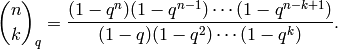
$\binom{n}{k}_q = \frac{(1-q^n)(1-q^{n-1})\cdots (1-q^{n-k+1})}{(1-q)(1-q^2)\cdots (1-q^k)}.$

EXAMPLES:

sage: gaussian_binomial(5,1)
q^4 + q^3 + q^2 + q + 1
sage: gaussian_binomial(5,1).subs(q=2)
31
sage: gaussian_binomial(5,1,2)
31

AUTHORS:

David Joyner and William Stein

sage.rings.arith.gcd(a, b=None, **kwargs)¶

The greatest common divisor of a and b, or if a is a list and b is omitted the greatest common divisor of all elements of a.

INPUT:

a,b - two elements of a ring with gcd or
a - a list or tuple of elements of a ring with gcd

Additional keyword arguments are passed to the respectively called methods.

EXAMPLES:

sage: GCD(97,100)
1
sage: GCD(97*10^15, 19^20*97^2)
97
sage: GCD(2/3, 4/3)
1
sage: GCD([2,4,6,8])
2
sage: GCD(srange(0,10000,10))  # fast  !!
10

Note that to take the gcd of $n$ elements for $n \not= 2$ you must put the elements into a list by enclosing them in [..]. Before #4988 the following wrongly returned 3 since the third parameter was just ignored:

sage: gcd(3,6,2)
...
TypeError: gcd() takes at most 2 arguments (3 given)
sage: gcd([3,6,2])
1

Similarly, giving just one element (which is not a list) gives an error:

sage: gcd(3)
...
TypeError: 'sage.rings.integer.Integer' object is not iterable

By convention, the gcd of the empty list is (the integer) 0:

sage: gcd([])
0
sage: type(gcd([]))
<type 'sage.rings.integer.Integer'>

sage.rings.arith.get_gcd(order)¶

Return the fastest gcd function for integers of size no larger than order.

EXAMPLES:

sage: sage.rings.arith.get_gcd(4000)
<built-in method gcd_int of sage.rings.fast_arith.arith_int object at ...>
sage: sage.rings.arith.get_gcd(400000)
<built-in method gcd_longlong of sage.rings.fast_arith.arith_llong object at ...>
sage: sage.rings.arith.get_gcd(4000000000)
<function gcd at ...>

sage.rings.arith.get_inverse_mod(order)¶

Return the fastest inverse_mod function for integers of size no larger than order.

EXAMPLES:

sage: sage.rings.arith.get_inverse_mod(6000)
<built-in method inverse_mod_int of sage.rings.fast_arith.arith_int object at ...>
sage: sage.rings.arith.get_inverse_mod(600000)
<built-in method inverse_mod_longlong of sage.rings.fast_arith.arith_llong object at ...>
sage: sage.rings.arith.get_inverse_mod(6000000000)
<function inverse_mod at ...>

sage.rings.arith.hilbert_conductor(a, b)¶

This is the product of all (finite) primes where the Hilbert symbol is -1. What is the same, this is the (reduced) discriminant of the quaternion algebra $(a,b)$ over $\QQ$ .

INPUT:

a, b – integers

OUTPUT:

squarefree positive integer

EXAMPLES:

sage: hilbert_conductor(-1, -1)
2
sage: hilbert_conductor(-1, -11)
11
sage: hilbert_conductor(-2, -5)
5
sage: hilbert_conductor(-3, -17)
17

AUTHOR:

Gonzalo Tornaria (2009-03-02)

sage.rings.arith.hilbert_conductor_inverse(d)¶

Finds a pair of integers $(a,b)$ such that hilbert_conductor(a,b) == d. The quaternion algebra $(a,b)$ over $\QQ$ will then have (reduced) discriminant $d$ .

INPUT:

d – square-free positive integer

OUTPUT: pair of integers

EXAMPLES:

sage: hilbert_conductor_inverse(2)
(-1, -1)
sage: hilbert_conductor_inverse(3)
(-1, -3)
sage: hilbert_conductor_inverse(6)
(-1, 3)
sage: hilbert_conductor_inverse(30)
(-3, -10)
sage: hilbert_conductor_inverse(4)
...
ValueError: d needs to be squarefree
sage: hilbert_conductor_inverse(-1)
...
ValueError: d needs to be positive

AUTHOR:

Gonzalo Tornaria (2009-03-02)

TESTS:

sage: for i in xrange(100):
...     d = ZZ.random_element(2**32).squarefree_part()
...     if hilbert_conductor(*hilbert_conductor_inverse(d)) != d:
...         print "hilbert_conductor_inverse failed for d =", d

sage.rings.arith.hilbert_symbol(a, b, p, algorithm='pari')¶

Returns 1 if $ax^2 + by^2$ $p$ -adically represents a nonzero square, otherwise returns $-1$ . If either a or b is 0, returns 0.

INPUT:

a, b - integers
p - integer; either prime or -1 (which represents the archimedean place)
algorithm - string
- 'pari' - (default) use the PARI C library
- 'direct' - use a Python implementation
- 'all' - use both PARI and direct and check that the results agree, then return the common answer

OUTPUT: integer (0, -1, or 1)

EXAMPLES:

sage: hilbert_symbol (-1, -1, -1, algorithm='all')
-1
sage: hilbert_symbol (2,3, 5, algorithm='all')
1
sage: hilbert_symbol (4, 3, 5, algorithm='all')
1
sage: hilbert_symbol (0, 3, 5, algorithm='all')
0
sage: hilbert_symbol (-1, -1, 2, algorithm='all')
-1
sage: hilbert_symbol (1, -1, 2, algorithm='all')
1
sage: hilbert_symbol (3, -1, 2, algorithm='all')
-1

sage: hilbert_symbol(QQ(-1)/QQ(4), -1, 2) == -1
True
sage: hilbert_symbol(QQ(-1)/QQ(4), -1, 3) == 1
True

AUTHORS:

William Stein and David Kohel (2006-01-05)

sage.rings.arith.integer_ceil(x)¶

Return the ceiling of x.

EXAMPLES:

sage: integer_ceil(5.4)
6

sage.rings.arith.integer_floor(x)¶

Return the largest integer $\leq x$ .

INPUT:

x - an object that has a floor method or is coercible to int

OUTPUT: an Integer

EXAMPLES:

sage: integer_floor(5.4)
5
sage: integer_floor(float(5.4))
5
sage: integer_floor(-5/2)
-3
sage: integer_floor(RDF(-5/2))
-3

sage.rings.arith.inverse_mod(a, m)¶

The inverse of the ring element a modulo m.

If no special inverse_mod is defined for the elements, it tries to coerce them into integers and perform the inversion there

sage: inverse_mod(7,1)
0
sage: inverse_mod(5,14)
3
sage: inverse_mod(3,-5)
2

sage.rings.arith.is_power_of_two(n)¶

This function returns True if and only if $n$ is a power of 2

INPUT:

n - integer

OUTPUT:

True - if n is a power of 2
False - if not

EXAMPLES:

sage: is_power_of_two(1024)
True

sage: is_power_of_two(1)
True

sage: is_power_of_two(24)
False

sage: is_power_of_two(0)
False

sage: is_power_of_two(-4)
False

AUTHORS:

Jaap Spies (2006-12-09)

sage.rings.arith.is_prime(n)¶

Returns True if $n$ is prime, and False otherwise.

AUTHORS:

Kevin Stueve kstueve@uw.edu (2010-01-17): delegated calculation to n.is_prime()

INPUT:

n - the object for which to determine primality

OUTPUT:

bool - True or False

EXAMPLES:

sage: is_prime(389)
True
sage: is_prime(2000)
False
sage: is_prime(2)
True
sage: is_prime(-1)   
False
sage: factor(-6)
-1 * 2 * 3
sage: is_prime(1)
False
sage: is_prime(-2)
False

ALGORITHM:

Calculation is delegated to the n.is_prime() method, or in special cases (e.g., Python int``s) to ``Integer(n).is_prime(). If an n.is_prime() method is not available, it otherwise raises a TypeError.

sage.rings.arith.is_prime_power(n, flag=0)¶

Returns True if $x$ is a prime power, and False otherwise. The result is proven correct - this is NOT a pseudo-primality test!.

INPUT:

n - an integer
flag (for primality testing) - int
- 0 (default): use a combination of algorithms.
- 1: certify primality using the Pocklington-Lehmer Test.
- 2: certify primality using the APRCL test.

EXAMPLES::

sage: is_prime_power(389)
True
sage: is_prime_power(2000)
False
sage: is_prime_power(2)
True
sage: is_prime_power(1024)
True
sage: is_prime_power(-1)   
False
sage: is_prime_power(1)
True
sage: is_prime_power(997^100)
True

sage.rings.arith.is_pseudoprime(n, flag=0)¶

Returns True if $x$ is a pseudo-prime, and False otherwise. The result is NOT proven correct - this is a pseudo-primality test!.

INPUT:

flag - int
- 0 (default): checks whether x is a Baillie-Pomerance- Selfridge-Wagstaff pseudo prime (strong Rabin-Miller pseudo prime for base 2, followed by strong Lucas test for the sequence (P,-1), P smallest positive integer such that $P^2 - 4$ is not a square mod x).
- >0: checks whether x is a strong Miller-Rabin pseudo prime for flag randomly chosen bases (with end-matching to catch square roots of -1).

OUTPUT:

bool - True or False

Note

We do not consider negatives of prime numbers as prime.

EXAMPLES::

sage: is_pseudoprime(389)
True
sage: is_pseudoprime(2000)
False
sage: is_pseudoprime(2)
True
sage: is_pseudoprime(-1)   
False
sage: factor(-6)
-1 * 2 * 3
sage: is_pseudoprime(1)
False
sage: is_pseudoprime(-2)
False

IMPLEMENTATION: Calls the PARI ispseudoprime function.

sage.rings.arith.is_square(n, root=False)¶

Returns whether or not n is square, and if n is a square also returns the square root. If n is not square, also returns None.

INPUT:

n - an integer
root - whether or not to also return a square root (default: False)

OUTPUT:

bool - whether or not a square
object - (optional) an actual square if found, and None otherwise.

EXAMPLES:

sage: is_square(2)
False
sage: is_square(4)    
True
sage: is_square(2.2)
True
sage: is_square(-2.2)
False
sage: is_square(CDF(-2.2))
True
sage: is_square((x-1)^2)
True

sage: is_square(4, True)
(True, 2)

sage.rings.arith.is_squarefree(n)¶

Returns True if and only if n is not divisible by the square of an integer > 1.

EXAMPLES:

sage: is_squarefree(100)
False
sage: is_squarefree(101)
True

sage.rings.arith.kronecker(x, y)¶

Synonym for kronecker_symbol().

The Kronecker symbol $(x|y)$ .

INPUT:

x - integer
y - integer

OUTPUT:

an integer

EXAMPLES:

sage: kronecker(3,5)
-1
sage: kronecker(3,15)
0
sage: kronecker(2,15)
1
sage: kronecker(-2,15)
-1
sage: kronecker(2/3,5)
1

sage.rings.arith.kronecker_symbol(x, y)¶

The Kronecker symbol $(x|y)$ .

INPUT:

x - integer
y - integer

EXAMPLES:

sage: kronecker_symbol(13,21)
-1
sage: kronecker_symbol(101,4)
1

IMPLEMENTATION: Using GMP.

sage.rings.arith.lcm(a, b=None)¶

The least common multiple of a and b, or if a is a list and b is omitted the least common multiple of all elements of a.

Note that LCM is an alias for lcm.

INPUT:

a,b - two elements of a ring with lcm or
a - a list or tuple of elements of a ring with lcm

EXAMPLES:

sage: lcm(97,100)
9700
sage: LCM(97,100)
9700
sage: LCM(0,2)
0
sage: LCM(-3,-5)
15
sage: LCM([1,2,3,4,5])
60
sage: v = LCM(range(1,10000))   # *very* fast!
sage: len(str(v))
4349

sage.rings.arith.legendre_symbol(x, p)¶

The Legendre symbol $(x|p)$ , for $p$ prime.

Note

The kronecker_symbol() command extends the Legendre symbol to composite moduli and $p=2$ .

INPUT:

x - integer
p - an odd prime number

EXAMPLES:

sage: legendre_symbol(2,3)
-1
sage: legendre_symbol(1,3)
1
sage: legendre_symbol(1,2)
...
ValueError: p must be odd
sage: legendre_symbol(2,15)
...
ValueError: p must be a prime
sage: kronecker_symbol(2,15)
1
sage: legendre_symbol(2/3,7)
-1

sage.rings.arith.mqrr_rational_reconstruction(u, m, T)¶

Maximal Quotient Rational Reconstruction.

For research purposes only - this is pure Python, so slow.

INPUT:

u, m, T - integers such that $m > u \ge 0$ , $T > 0$ .

OUTPUT:

Either integers $n,d$ such that $d>0$ , $\mathop{\mathrm{gcd}}(n,d)=1$ , $n/d=u \bmod m$ , and $T \cdot d \cdot |n| < m$ , or None.

Reference: Monagan, Maximal Quotient Rational Reconstruction: An Almost Optimal Algorithm for Rational Reconstruction (page 11)

This algorithm is probabilistic.

EXAMPLES:

sage: mqrr_rational_reconstruction(21,3100,13)
(21, 1)

sage.rings.arith.multinomial(*ks)¶

Return the multinomial coefficient

INPUT:

An arbitrary number of integer arguments $k_1,\dots,k_n$
A list of integers $[k_1,\dots,k_n]$

OUTPUT:

Returns the integer:

$\binom{k_1 + \cdots + k_n}{k_1, \cdots, k_n} =\frac{\left(\sum_{i=1}^n k_i\right)!}{\prod_{i=1}^n k_i!} = \prod_{i=1}^n \binom{\sum_{j=1}^i k_j}{k_i}$

EXAMPLES:

sage: multinomial(0, 0, 2, 1, 0, 0)
3
sage: multinomial([0, 0, 2, 1, 0, 0])
3
sage: multinomial(3, 2)
10
sage: multinomial(2^30, 2, 1)
618970023101454657175683075
sage: multinomial([2^30, 2, 1])
618970023101454657175683075

AUTHORS:

Gabriel Ebner

sage.rings.arith.multinomial_coefficients(m, n, _tuple=<type 'tuple'>, _zip=<built-in function zip>)¶

Return a dictionary containing pairs $\{(k_1,k_2,...,k_m) : C_{k,n}\}$ where $C_{k,n}$ are multinomial coefficients such that $n = k_1 + k_2 + ...+ k_m$ .

INPUT:

m - integer
n - integer
_tuple, _zip - hacks for speed; don’t set these as a user.

OUTPUT: dict

EXAMPLES:

sage: sorted(multinomial_coefficients(2,5).items())
[((0, 5), 1), ((1, 4), 5), ((2, 3), 10), ((3, 2), 10), ((4, 1), 5), ((5, 0), 1)]

Notice that these are the coefficients of $(x+y)^5$ :

sage: R.<x,y> = QQ[]
sage: (x+y)^5
x^5 + 5*x^4*y + 10*x^3*y^2 + 10*x^2*y^3 + 5*x*y^4 + y^5

sage: sorted(multinomial_coefficients(3,2).items())
[((0, 0, 2), 1), ((0, 1, 1), 2), ((0, 2, 0), 1), ((1, 0, 1), 2), ((1, 1, 0), 2), ((2, 0, 0), 1)]

ALGORITHM: The algorithm we implement for computing the multinomial coefficients is based on the following result:

Consider a polynomial and its $n$ -th exponent:

$P(x) = \sum_{i=0}^m p_i x^k$

$P(x)^n = \sum_{k=0}^{m n} a(n,k) x^k$

We compute the coefficients $a(n,k)$ using the J.C.P. Miller Pure Recurrence [see D.E.Knuth, Seminumerical Algorithms, The art of Computer Programming v.2, Addison Wesley, Reading, 1981].

$a(n,k) = 1/(k p_0) \sum_{i=1}^m p_i ((n+1)i-k) a(n,k-i),$

where $a(n,0) = p_0^n$ .

AUTHORS:

Pearu Peterson

sage.rings.arith.next_prime(n, proof=None)¶

The next prime greater than the integer n. If n is prime, then this function does not return n, but the next prime after n. If the optional argument proof is False, this function only returns a pseudo-prime, as defined by the PARI nextprime function. If it is None, uses the global default (see sage.structure.proof.proof)

INPUT:

n - integer
proof - bool or None (default: None)

EXAMPLES:

sage: next_prime(-100)
2
sage: next_prime(1)
2
sage: next_prime(2)
3
sage: next_prime(3)
5
sage: next_prime(4)
5

Notice that the next_prime(5) is not 5 but 7.

sage: next_prime(5)
7
sage: next_prime(2004)
2011

sage.rings.arith.next_prime_power(n)¶

The next prime power greater than the integer n. If n is a prime power, then this function does not return n, but the next prime power after n.

EXAMPLES:

sage: next_prime_power(-10)
1
sage: is_prime_power(1)
True
sage: next_prime_power(0)
1
sage: next_prime_power(1)
2
sage: next_prime_power(2)
3
sage: next_prime_power(10)
11
sage: next_prime_power(7)
8
sage: next_prime_power(99)
101

sage.rings.arith.next_probable_prime(n)¶

Returns the next probable prime after self, as determined by PARI.

INPUT:

n - an integer

EXAMPLES:

sage: next_probable_prime(-100)
2
sage: next_probable_prime(19)
23
sage: next_probable_prime(int(999999999))
1000000007
sage: next_probable_prime(2^768)
1552518092300708935148979488462502555256886017116696611139052038026050952686376886330878408828646477950487730697131073206171580044114814391444287275041181139204454976020849905550265285631598444825262999193716468750892846853816058039

sage.rings.arith.nth_prime(n)¶

EXAMPLES:

sage: nth_prime(3)
5
sage: nth_prime(10)
29

sage: nth_prime(0)
...
ValueError: nth prime meaningless for non-positive n (=0)

sage.rings.arith.number_of_divisors(n)¶

Return the number of divisors of the integer n.

INPUT:

n - a nonzero integer

OUTPUT:

an integer, the number of divisors of n

EXAMPLES:

sage: number_of_divisors(100)
9
sage: number_of_divisors(-720)
30

sage.rings.arith.odd_part(n)¶

The odd part of the integer $n$ . This is $n / 2^v$ , where $v = \mathrm{valuation}(n,2)$ .

EXAMPLES:

sage: odd_part(5)
5
sage: odd_part(4)
1
sage: odd_part(factorial(31))
122529844256906551386796875

sage.rings.arith.power_mod(a, n, m)¶

The n-th power of a modulo the integer m.

EXAMPLES:

sage: power_mod(0,0,5)
...
ArithmeticError: 0^0 is undefined.
sage: power_mod(2,390,391)
285
sage: power_mod(2,-1,7)
4
sage: power_mod(11,1,7)
4
sage: R.<x> = ZZ[]
sage: power_mod(3*x, 10, 7)
4*x^10

sage: power_mod(11,1,0)
...
ZeroDivisionError: modulus must be nonzero.

sage.rings.arith.previous_prime(n)¶

The largest prime < n. The result is provably correct. If n <= 1, this function raises a ValueError.

EXAMPLES:

sage: previous_prime(10)
7
sage: previous_prime(7)
5
sage: previous_prime(8)
7
sage: previous_prime(7)
5
sage: previous_prime(5)
3
sage: previous_prime(3)
2
sage: previous_prime(2)
...
ValueError: no previous prime        
sage: previous_prime(1)
...
ValueError: no previous prime        
sage: previous_prime(-20)
...
ValueError: no previous prime

sage.rings.arith.previous_prime_power(n)¶

The largest prime power $< n$ . The result is provably correct. If $n \leq 2$ , this function returns $-x$ , where $x$ is prime power and $-x < n$ and no larger negative of a prime power has this property.

EXAMPLES:

sage: previous_prime_power(2)
1
sage: previous_prime_power(10)
9
sage: previous_prime_power(7)
5
sage: previous_prime_power(127)
125    

sage: previous_prime_power(0)
...
ValueError: no previous prime power
sage: previous_prime_power(1)
...
ValueError: no previous prime power

sage: n = previous_prime_power(2^16 - 1)
sage: while is_prime(n): 
...    n = previous_prime_power(n)
sage: factor(n)
251^2

sage.rings.arith.prime_divisors(n)¶

The prime divisors of the integer n, sorted in increasing order. If n is negative, we do not include -1 among the prime divisors, since -1 is not a prime number.

EXAMPLES:

sage: prime_divisors(1)
[]
sage: prime_divisors(100)
[2, 5]
sage: prime_divisors(-100)
[2, 5]
sage: prime_divisors(2004)
[2, 3, 167]

sage.rings.arith.prime_factors(n)¶

The prime divisors of the integer n, sorted in increasing order. If n is negative, we do not include -1 among the prime divisors, since -1 is not a prime number.

EXAMPLES:

sage: prime_divisors(1)
[]
sage: prime_divisors(100)
[2, 5]
sage: prime_divisors(-100)
[2, 5]
sage: prime_divisors(2004)
[2, 3, 167]

sage.rings.arith.prime_powers(start, stop=None)¶

List of all positive primes powers between start and stop-1, inclusive. If the second argument is omitted, returns the primes up to the first argument.

EXAMPLES:

sage: prime_powers(20)
[1, 2, 3, 4, 5, 7, 8, 9, 11, 13, 16, 17, 19]
sage: len(prime_powers(1000))
194
sage: len(prime_range(1000))
168
sage: a = [z for z in range(95,1234) if is_prime_power(z)]
sage: b = prime_powers(95,1234)
sage: len(b)
194
sage: len(a)
194
sage: a[:10]
[97, 101, 103, 107, 109, 113, 121, 125, 127, 128]
sage: b[:10]
[97, 101, 103, 107, 109, 113, 121, 125, 127, 128]
sage: a == b
True

TESTS:

sage: v = prime_powers(10) 
sage: type(v[0])      # trac #922
<type 'sage.rings.integer.Integer'>

sage.rings.arith.prime_to_m_part(n, m)¶

Returns the prime-to-m part of n, i.e., the largest divisor of n that is coprime to m.

INPUT:

n - Integer (nonzero)
m - Integer

OUTPUT: Integer

EXAMPLES:

sage: z = 43434
sage: z.prime_to_m_part(20)
21717

sage.rings.arith.primes(start, stop=None)¶

Returns an iterator over all primes between start and stop-1, inclusive. This is much slower than prime_range, but potentially uses less memory.

This command is like the xrange command, except it only iterates over primes. In some cases it is better to use primes than prime_range, because primes does not build a list of all primes in the range in memory all at once. However it is potentially much slower since it simply calls the next_prime function repeatedly, and next_prime is slow, partly because it proves correctness.

EXAMPLES:

sage: for p in primes(5,10):
...     print p
...
5
7
sage: list(primes(11))
[2, 3, 5, 7]
sage: list(primes(10000000000, 10000000100))
[10000000019, 10000000033, 10000000061, 10000000069, 10000000097]

sage.rings.arith.primes_first_n(n, leave_pari=False)¶

Return the first $n$ primes.

INPUT:

$n$ - a nonnegative integer

OUTPUT:

a list of the first $n$ prime numbers.

EXAMPLES:

sage: primes_first_n(10)
[2, 3, 5, 7, 11, 13, 17, 19, 23, 29]
sage: len(primes_first_n(1000))
1000
sage: primes_first_n(0)
[]

sage.rings.arith.primitive_root(n)¶

Return a generator for the multiplicative group of integers modulo $n$ , if one exists.

EXAMPLES:

sage: primitive_root(23)
5
sage: print [primitive_root(p) for p in primes(100)]
[1, 2, 2, 3, 2, 2, 3, 2, 5, 2, 3, 2, 6, 3, 5, 2, 2, 2, 2, 7, 5, 3, 2, 3, 5]

sage.rings.arith.quadratic_residues(n)¶

Return a sorted list of all squares modulo the integer $n$ in the range $0\leq x < |n|$ .

EXAMPLES:

sage: quadratic_residues(11)
[0, 1, 3, 4, 5, 9]
sage: quadratic_residues(1)
[0]
sage: quadratic_residues(2)
[0, 1]
sage: quadratic_residues(8)
[0, 1, 4]
sage: quadratic_residues(-10)
[0, 1, 4, 5, 6, 9]
sage: v = quadratic_residues(1000); len(v);
159

sage.rings.arith.random_prime(n, proof=None, lbound=2)¶

Returns a random prime p between $lbound$ and n (i.e. $lbound <= p <= n$ ). The returned prime is chosen uniformly at random from the set of prime numbers less than or equal to n.

INPUT:

n - an integer >= 2.
proof - bool or None (default: None) If False, the function uses a pseudo-primality test, which is much faster for really big numbers but does not provide a proof of primality. If None, uses the global default (see sage.structure.proof.proof)
lbound - an integer >= 2 lower bound for the chosen primes

EXAMPLES:

sage: random_prime(100000)
88237
sage: random_prime(2)
2

TESTS:

sage: type(random_prime(2))
<type 'sage.rings.integer.Integer'>
sage: type(random_prime(100))
<type 'sage.rings.integer.Integer'>        

AUTHORS:

Jon Hanke (2006-08-08): with standard Stein cleanup
Jonathan Bober (2007-03-17)

sage.rings.arith.rational_reconstruction(a, m, algorithm='fast')¶

This function tries to compute $x/y$ , where $x/y$ is a rational number in lowest terms such that the reduction of $x/y$ modulo $m$ is equal to $a$ and the absolute values of $x$ and $y$ are both $\le \sqrt{m/2}$ . If such $x/y$ exists, that pair is unique and this function returns it. If no such pair exists, this function raises ZeroDivisionError.

An efficient algorithm for computing rational reconstruction is very similar to the extended Euclidean algorithm. For more details, see Knuth, Vol 2, 3rd ed, pages 656-657.

INPUT:

a - an integer
m - a modulus
algorithm - (default: ‘fast’)
- 'fast' - a fast compiled implementation
- 'python' - a slow pure python implementation

OUTPUT:

Numerator and denominator $n$ , $d$ of the unique rational number $r=n/d$ , if it exists, with $n$ and $|d| \le \sqrt{N/2}$ . Return $(0,0)$ if no such number exists.

The algorithm for rational reconstruction is described (with a complete nontrivial proof) on pages 656-657 of Knuth, Vol 2, 3rd ed. as the solution to exercise 51 on page 379. See in particular the conclusion paragraph right in the middle of page 657, which describes the algorithm thus:

This discussion proves that the problem can be solved efficiently by applying Algorithm 4.5.2X with $u=m$ and $v=a$ , but with the following replacement for step X2: If $v3 \le \sqrt{m/2}$ , the algorithm terminates. The pair $(x,y)=(|v2|,v3*\mathrm{sign}(v2))$ is then the unique solution, provided that $x$ and $y$ are coprime and $x \le \sqrt{m/2}$ ; otherwise there is no solution. (Alg 4.5.2X is the extended Euclidean algorithm.)

Knuth remarks that this algorithm is due to Wang, Kornerup, and Gregory from around 1983.

EXAMPLES:

sage: m = 100000
sage: (119*inverse_mod(53,m))%m
11323
sage: rational_reconstruction(11323,m)
119/53

sage: rational_reconstruction(400,1000)
...
ValueError: Rational reconstruction of 400 (mod 1000) does not exist.

sage: rational_reconstruction(3,292393, algorithm='python')
3
sage: a = Integers(292393)(45/97); a
204977
sage: rational_reconstruction(a,292393, algorithm='python')
45/97
sage: a = Integers(292393)(45/97); a
204977
sage: rational_reconstruction(a,292393, algorithm='fast')
45/97
sage: rational_reconstruction(293048,292393, algorithm='fast')
...
ValueError: Rational reconstruction of 655 (mod 292393) does not exist.
sage: rational_reconstruction(293048,292393, algorithm='python')
...
ValueError: Rational reconstruction of 655 (mod 292393) does not exist.

sage.rings.arith.rising_factorial(x, a)¶

Returns the rising factorial $(x)^a$ .

The notation in the literature is a mess: often $(x)^a$ , but there are many other notations: GKP: Concrete Mathematics uses $x^{\overline{a}}$ .

The rising factorial is also known as the Pochhammer symbol, see Maple and Mathematica.

Definition: for integer $a \ge 0$ we have $x(x+1) \cdots (x+a-1)$ . In all other cases we use the GAMMA-function: $\frac {\Gamma(x+a)} {\Gamma(x)}$ .

INPUT:

x - element of a ring
a - a non-negative integer or
x and a - any numbers

OUTPUT: the rising factorial

EXAMPLES:

sage: rising_factorial(10,3)
1320  

sage: rising_factorial(10,RR('3.0'))
1320.00000000000

sage: rising_factorial(10,RR('3.3'))
2826.38895824964

sage: a = rising_factorial(1+I, I); a
gamma(2*I + 1)/gamma(I + 1)
sage: CC(a)
0.266816390637832 + 0.122783354006372*I

sage: a = rising_factorial(I, 4); a
-10

See falling_factorial(I, 4).

sage: x = polygen(ZZ)
sage: rising_factorial(x, 4)
x^4 + 6*x^3 + 11*x^2 + 6*x 

AUTHORS:

Jaap Spies (2006-03-05)

sage.rings.arith.sort_complex_numbers_for_display(nums)¶

Given a list of complex numbers (or a list of tuples, where the first element of each tuple is a complex number), we sort the list in a “pretty” order. First come the real numbers (with zero imaginary part), then the complex numbers sorted according to their real part. If two complex numbers have a real part which is sufficiently close, then they are sorted according to their imaginary part.

This is not a useful function mathematically (not least because there’s no principled way to determine whether the real components should be treated as equal or not). It is called by various polynomial root-finders; its purpose is to make doctest printing more reproducible.

We deliberately choose a cumbersome name for this function to discourage use, since it is mathematically meaningless.

EXAMPLES:

sage: import sage.rings.arith
sage: sort_c = sort_complex_numbers_for_display
sage: nums = [CDF(i) for i in range(3)]
sage: for i in range(3):
...       nums.append(CDF(i + RDF.random_element(-3e-11, 3e-11),
...                       RDF.random_element()))
...       nums.append(CDF(i + RDF.random_element(-3e-11, 3e-11),
...                       RDF.random_element()))
sage: shuffle(nums)
sage: sort_c(nums)
[0, 1.0, 2.0, -2.862406201e-11 - 0.708874026302*I, 2.2108362707e-11 - 0.436810529675*I, 1.00000000001 - 0.758765473764*I, 0.999999999976 - 0.723896589334*I, 1.99999999999 - 0.456080101207*I, 1.99999999999 + 0.609083628313*I]

sage.rings.arith.squarefree_divisors(x)¶

Iterator over the squarefree divisors (up to units) of the element x.

Depends on the output of the prime_divisors function.

INPUT:

x -- an element of any ring for which the prime_divisors
     function works.

EXAMPLES:

sage: list(squarefree_divisors(7))
[1, 7]
sage: list(squarefree_divisors(6))
[1, 2, 3, 6]
sage: list(squarefree_divisors(12))
[1, 2, 3, 6]

sage.rings.arith.subfactorial(n)¶

Subfactorial or rencontres numbers, or derangements: number of permutations of $n$ elements with no fixed points.

INPUT:

n - non negative integer

OUTPUT:

integer - function value

EXAMPLES:

sage: subfactorial(0)
1
sage: subfactorial(1)
0
sage: subfactorial(8)
14833

AUTHORS:

Jaap Spies (2007-01-23)

sage.rings.arith.trial_division(n, bound=None)¶

Return the smallest prime divisor <= bound of the positive integer n, or n if there is no such prime. If the optional argument bound is omitted, then bound <= n.

INPUT:

n - a positive integer
bound - (optional) a positive integer

OUTPUT:

int - a prime p=bound that divides n, or n if there is no such prime.

EXAMPLES:

sage: trial_division(15)
3
sage: trial_division(91)
7
sage: trial_division(11)
11
sage: trial_division(387833, 300)   
387833
sage: # 300 is not big enough to split off a 
sage: # factor, but 400 is.
sage: trial_division(387833, 400)  
389

sage.rings.arith.two_squares(n, algorithm='gap')¶

Write the integer n as a sum of two integer squares if possible; otherwise raise a ValueError.

EXAMPLES:

sage: two_squares(389)
(10, 17)
sage: two_squares(7)
...
ValueError: 7 is not a sum of two squares
sage: a,b = two_squares(2009); a,b
(28, 35)
sage: a^2 + b^2
2009

TODO: Create an implementation using PARI’s continued fraction implementation.

sage.rings.arith.valuation(m, p)¶

The exact power of p that divides m.

m should be an integer or rational (but maybe other types work too.)

This actually just calls the m.valuation() method.

If m is 0, this function returns rings.infinity.

EXAMPLES:

sage: valuation(512,2)
9
sage: valuation(1,2)
0
sage: valuation(5/9, 3)
-2

Valuation of 0 is defined, but valuation with respect to 0 is not:

sage: valuation(0,7)
+Infinity
sage: valuation(3,0)
...
ValueError: You can only compute the valuation with respect to a integer larger than 1.

Here are some other examples:

sage: valuation(100,10)
2
sage: valuation(200,10)
2
sage: valuation(243,3)
5
sage: valuation(243*10007,3)
5
sage: valuation(243*10007,10007)
1

sage.rings.arith.xgcd(a, b)¶

Return a triple (g,s,t) such that $g = s\cdot a+t\cdot b = \gcd(a,b)$ .

Note

One exception is if $a$ and $b$ are not in a PID, e.g., they are both polynomials over the integers, then this function can’t in general return (g,s,t) as above, since they need not exist. Instead, over the integers, we first multiply $g$ by a divisor of the resultant of $a/g$ and $b/g$ , up to sign.

INPUT:

a, b - integers or univariate polynomials (or any type with an xgcd method).

OUTPUT:

g, s, t - such that $g = s\cdot a + t\cdot b$

Note

There is no guarantee that the returned cofactors (s and t) are minimal. In the integer case, see sage.rings.integer.Integer._xgcd() for minimal cofactors.

EXAMPLES:

sage: xgcd(56, 44)
(4, 4, -5)
sage: 4*56 + (-5)*44
4
sage: g, a, b = xgcd(5/1, 7/1); g, a, b
(1, 3, -2)
sage: a*(5/1) + b*(7/1) == g
True
sage: x = polygen(QQ)
sage: xgcd(x^3 - 1, x^2 - 1)
(x - 1, 1, -x)
sage: K.<g> = NumberField(x^2-3)
sage: R.<a,b> = K[]
sage: S.<y> = R.fraction_field()[]
sage: xgcd(y^2, a*y+b)
(1, a^2/b^2, ((-a)/b^2)*y + 1/b)
sage: xgcd((b+g)*y^2, (a+g)*y+b)
(1, (a^2 + (2*g)*a + 3)/(b^3 + (g)*b^2), ((-a + (-g))/b^2)*y + 1/b)

We compute an xgcd over the integers, where the linear combination is not the gcd but the resultant:

sage: R.<x> = ZZ[]
sage: gcd(2*x*(x-1), x^2)
x
sage: xgcd(2*x*(x-1), x^2)
(2*x, -1, 2)
sage: (2*(x-1)).resultant(x)
2

sage.rings.arith.xlcm(m, n)¶

Extended lcm function: given two positive integers $m,n$ , returns a triple $(l,m_1,n_1)$ such that $l=\mathop{\mathrm{lcm}}(m,n)=m_1 \cdot n_1$ where $m_1|m$ , $n_1|n$ and $\gcd(m_1,n_1)=1$ , all with no factorization.