AUTHOR:
Solves the bin packing problem.
The Bin Packing problem is the following :
Given a list of items of weights  and a real value
  , what is
the least number of bins such that all the items can be put in the
bins, while keeping sure that each bin contains a weight of at most ?
, what is
the least number of bins such that all the items can be put in the
bins, while keeping sure that each bin contains a weight of at most ?
For more informations : http://en.wikipedia.org/wiki/Bin_packing_problem
 bins ?
INPUT:
 bins if possible, and raises an
exception otherwise.
bins if possible, and raises an
exception otherwise.OUTPUT:
A list of lists, each member corresponding to a box and containing the list of the weights inside it. If there is no solution, an exception is raised (this can only happen when k is specified or if maximum is less that the size of one item).
EXAMPLES:
Trying to find the minimum amount of boxes for 5 items of weights
 :
:
sage: from sage.numerical.optimize import binpacking
sage: values = [1/5, 1/3, 2/3, 3/4, 5/7]
sage: bins = binpacking(values)
sage: len(bins)
3
Checking the bins are of correct size
sage: all([ sum(b)<= 1 for b in bins ])
True
Checking every item is in a bin
sage: b1, b2, b3 = bins
sage: all([ (v in b1 or v in b2 or v in b3) for v in values ])
True
One way to use only three boxes (which is best possible) is to put
 together in a box,
  in another, and
  by itself in the third one.
Of course, we can also check that there is no solution using only two boxes
sage: from sage.numerical.optimize import binpacking
sage: binpacking([0.2,0.3,0.8,0.9], k=2)
...
ValueError: This problem has no solution !
Finds numerical estimates for the parameters of the function model to give a best fit to data.
INPUT:
![[[x_{1,1}, x_{1,2}, \ldots, x_{1,k}, f_1],
[x_{2,1}, x_{2,2}, \ldots, x_{2,k}, f_2],
\ldots,
[x_{n,1}, x_{n,2}, \ldots, x_{n,k}, f_n]]](../../_images/math/d09fa9b0f51244c6d469e61e937d485b6dbb9960.png) given as either a list of
lists, matrix, or numpy array.
given as either a list of
lists, matrix, or numpy array. and free parameters
 ., given as either a list, tuple,
vector or numpy array. If None, the default estimate for each
parameter is
., given as either a list, tuple,
vector or numpy array. If None, the default estimate for each
parameter is  .. If model is a symbolic function it is
ignored, and the free parameters of the symbolic function are used.. If model is a symbolic function it is
ignored, and the variables of the symbolic function are used.
.. If model is a symbolic function it is
ignored, and the free parameters of the symbolic function are used.. If model is a symbolic function it is
ignored, and the variables of the symbolic function are used.EXAMPLES:
First we create some data points of a sine function with some random perturbations:
sage: data = [(i, 1.2 * sin(0.5*i-0.2) + 0.1 * normalvariate(0, 1)) for i in xsrange(0, 4*pi, 0.2)]
sage: var('a, b, c, x')
(a, b, c, x)
We define a function with free parameters  ,
,  and
and  :
:
sage: model(x) = a * sin(b * x - c)
We search for the parameters that give the best fit to the data:
sage: find_fit(data, model)
[a == 1.21..., b == 0.49..., c == 0.19...]
We can also use a Python function for the model:
sage: def f(x, a, b, c): return a * sin(b * x - c)
sage: fit = find_fit(data, f, parameters = [a, b, c], variables = [x], solution_dict = True)
sage: fit[a], fit[b], fit[c]
(1.21..., 0.49..., 0.19...)
We search for a formula for the  -th prime number:
sage: dataprime = [(i, nth_prime(i)) for i in xrange(1, 5000, 100)]
sage: find_fit(dataprime, a * x * log(b * x), parameters = [a, b], variables = [x])
[a == 1.11..., b == 1.24...]
ALGORITHM:
Uses scipy.optimize.leastsq which in turn uses MINPACK’s lmdif and lmder algorithms.
Numerically find the maximum of the expression  on the interval
![[a,b]](../../_images/math/8ecbd1ba3da8f2adef66a63f2ab32c47e63fa734.png) (or
(or ![[b,a]](../../_images/math/a5aa84566486814ea5e952727df5d17a1b168480.png) ) along with the point at which the maximum is attained.
) along with the point at which the maximum is attained.
See the documentation for find_minimum_on_interval() for more details.
EXAMPLES:
sage: f = lambda x: x*cos(x)
sage: find_maximum_on_interval(f, 0,5)
(0.561096338191..., 0.8603335890...)
sage: find_maximum_on_interval(f, 0,5, tol=0.1, maxfun=10)
(0.561090323458..., 0.857926501456...)
Numerically find the minimum of the expression f on the
interval (or ) and the point at which it attains that
minimum. Note that f must be a function of (at most) one
variable.
INPUT:
OUTPUT:
EXAMPLES:
sage: f = lambda x: x*cos(x)
sage: find_minimum_on_interval(f, 1, 5)
(-3.28837139559..., 3.4256184695...)
sage: find_minimum_on_interval(f, 1, 5, tol=1e-3)
(-3.28837136189098..., 3.42575079030572...)
sage: find_minimum_on_interval(f, 1, 5, tol=1e-2, maxfun=10)
(-3.28837084598..., 3.4250840220...)
sage: show(plot(f, 0, 20))
sage: find_minimum_on_interval(f, 1, 15)
(-9.4772942594..., 9.5293344109...)
ALGORITHM:
Uses scipy.optimize.fminbound which uses Brent’s method.
AUTHOR:
Numerically find a root of f on the closed interval
(or ) if possible, where f is a function in the one variable.
INPUT:
 .
The routine modifies this to take into account the relative precision
of doubles..
.
The routine modifies this to take into account the relative precision
of doubles..EXAMPLES:
An example involving an algebraic polynomial function:
sage: R.<x> = QQ[]
sage: f = (x+17)*(x-3)*(x-1/8)^3
sage: find_root(f, 0,4)
2.9999999999999951
sage: find_root(f, 0,1)  # note -- precision of answer isn't very good on some machines.
0.124999...
sage: find_root(f, -20,-10)
-17.0
In Pomerance book on primes he asserts that the famous Riemann
Hypothesis is equivalent to the statement that the function  defined below is positive for all
  :
:
sage: def f(x):
...       return sqrt(x) * log(x) - abs(Li(x) - prime_pi(x))
We find where equals, i.e., what value that is slightly smaller
than  that could have been used in the formulation of the Riemann
Hypothesis:
that could have been used in the formulation of the Riemann
Hypothesis:
sage: find_root(f, 2, 4, rtol=0.0001)
2.0082590205656166
This agrees with the plot:
sage: plot(f,2,2.01)
Solves the dual linear programs:
 subject to
  ,
,  , and
, and  where
where
 denotes transpose.
 subject to
  and
and  .
.INPUT:
These can be over any field that can be turned into a floating point number.
OUTPUT:
A dictionary sol with keys x, s, y, z corresponding to the variables above:
EXAMPLES:
First, we minimize  subject to
  ,
,
 ,
,  , and
, and  :
:
sage: c=vector(RDF,[-4,-5])
sage: G=matrix(RDF,[[2,1],[1,2],[-1,0],[0,-1]])
sage: h=vector(RDF,[3,3,0,0])
sage: sol=linear_program(c,G,h)
sage: sol['x']
(0.999..., 1.000...)
Next, we maximize  subject to
 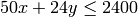 ,
,
 ,
,  , and
, and  :
:
sage: v=vector([-1.0,-1.0,-1.0])
sage: m=matrix([[50.0,24.0,0.0],[30.0,33.0,0.0],[-1.0,0.0,0.0],[0.0,-1.0,0.0],[0.0,0.0,1.0],[0.0,0.0,-1.0]])
sage: h=vector([2400.0,2100.0,-45.0,-5.0,1.0,-1.0])
sage: sol=linear_program(v,m,h)
sage: sol['x']
(45.000000..., 6.2499999...3, 1.00000000...)
This function is an interface to a variety of algorithms for computing the minimum of a function of several variables.
INPUT:
func – Either a symbolic function or a Python function whose
argument is a tuple with components
x0 – Initial point for finding minimum.
gradient – Optional gradient function. This will be computed automatically for symbolic functions. For Python functions, it allows the use of algorithms requiring derivatives. It should accept a tuple of arguments and return a NumPy array containing the partial derivatives at that point.
hessian – Optional hessian function. This will be computed automatically for symbolic functions. For Python functions, it allows the use of algorithms requiring derivatives. It should accept a tuple of arguments and return a NumPy array containing the second partial derivatives of the function.
algorithm – String specifying algorithm to use. Options are 'default' (for Python functions, the simplex method is the default) (for symbolic functions bfgs is the default):
- 'simplex'
- 'powell'
- 'bfgs' – (broyden-fletcher-goldfarb-shannon) requires gradient
- 'cg' – (conjugate-gradient) requires gradient
- 'ncg' – (newton-conjugate gradient) requires gradient and hessian
EXAMPLES:
sage: vars=var('x y z')
sage: f=100*(y-x^2)^2+(1-x)^2+100*(z-y^2)^2+(1-y)^2
sage: minimize(f,[.1,.3,.4],disp=0)
(1.00..., 1.00..., 1.00...)

sage: minimize(f,[.1,.3,.4],algorithm="ncg",disp=0)
(0.9999999..., 0.999999..., 0.999999...)
Same example with just Python functions:
sage: def rosen(x): # The Rosenbrock function
...      return sum(100.0r*(x[1r:]-x[:-1r]**2.0r)**2.0r + (1r-x[:-1r])**2.0r)
sage: minimize(rosen,[.1,.3,.4],disp=0)
(1.00..., 1.00..., 1.00...)
Same example with a pure Python function and a Python function to compute the gradient:
sage: def rosen(x): # The Rosenbrock function
...      return sum(100.0r*(x[1r:]-x[:-1r]**2.0r)**2.0r + (1r-x[:-1r])**2.0r)
sage: import numpy
sage: from numpy import zeros
sage: def rosen_der(x):
...      xm = x[1r:-1r]
...      xm_m1 = x[:-2r]
...      xm_p1 = x[2r:]
...      der = zeros(x.shape,dtype=float)
...      der[1r:-1r] = 200r*(xm-xm_m1**2r) - 400r*(xm_p1 - xm**2r)*xm - 2r*(1r-xm)
...      der[0] = -400r*x[0r]*(x[1r]-x[0r]**2r) - 2r*(1r-x[0])
...      der[-1] = 200r*(x[-1r]-x[-2r]**2r)
...      return der
sage: minimize(rosen,[.1,.3,.4],gradient=rosen_der,algorithm="bfgs",disp=0)
(1.00...,  1.00..., 1.00...)
Minimize a function with constraints.
INPUT:
components
(assuming variables). If the constraints are specified as a list
of intervals and there are no constraints for a given variable, that
component can be (None, None).EXAMPLES:
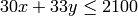
Let us maximize  subject to the following constraints:
, , ,
and :
subject to the following constraints:
, , ,
and :
sage: y = var('y')
sage: f = lambda p: -p[0]-p[1]+50
sage: c_1 = lambda p: p[0]-45
sage: c_2 = lambda p: p[1]-5
sage: c_3 = lambda p: -50*p[0]-24*p[1]+2400
sage: c_4 = lambda p: -30*p[0]-33*p[1]+2100
sage: a = minimize_constrained(f,[c_1,c_2,c_3,c_4],[2,3])
sage: a
(45.0, 6.25)
Let’s find a minimum of  :
:
sage: x,y = var('x y')
sage: f = sin(x*y)
sage: minimize_constrained(f, [(None,None),(4,10)],[5,5])
(4.8..., 4.8...)
Check, if L-BFGS-B finds the same minimum:
sage: minimize_constrained(f, [(None,None),(4,10)],[5,5], algorithm='l-bfgs-b')
(4.7..., 4.9...)
Rosenbrock function, [http://en.wikipedia.org/wiki/Rosenbrock_function]:
sage: from scipy.optimize import rosen, rosen_der
sage: minimize_constrained(rosen, [(-50,-10),(5,10)],[1,1],gradient=rosen_der,algorithm='l-bfgs-b')
(-10.0, 10.0)
sage: minimize_constrained(rosen, [(-50,-10),(5,10)],[1,1],algorithm='l-bfgs-b')
(-10.0, 10.0)
REFERENCES:
| [ZBN97] | C. Zhu, R. H. Byrd and J. Nocedal. L-BFGS-B: Algorithm 778: L-BFGS-B, FORTRAN routines for large scale bound constrained optimization. ACM Transactions on Mathematical Software, Vol 23, Num. 4, pp.550–560, 1997. |
