Navigation
- index
- modules |
- next |
- previous |
- Sage Reference v4.5.1 »
- Graph Theory »

AUTHORS:
This class performs randomized testing for all_graph_colorings.
Since everything else in this file is derived from
all_graph_colorings, this is a pretty good randomized tester for
the entire file. Note that for a graph  , G.chromatic_polynomial()
uses an entirely different algorithm, so we provide a good,
independent test.
, G.chromatic_polynomial()
uses an entirely different algorithm, so we provide a good,
independent test.
Calls self.random_all_graph_colorings(). In the future, if other methods are added, it should call them, too.
TESTS:
sage: from sage.graphs.graph_coloring import Test
sage: Test().random(1)
Verifies the results of all_graph_colorings() in three ways:
 (where
  is the chromatic
polynomial of the graph being tested)
is the chromatic
polynomial of the graph being tested)TESTS:
sage: from sage.graphs.graph_coloring import Test
sage: Test().random_all_graph_colorings(1)
Computes an acyclic edge coloring of the current graph.
An edge coloring of a graph is a assignment of colors to the edges of a graph such that :
 , the union of the edges
colored with
, the union of the edges
colored with  or
or  is a forest.
The least number of colors such that such a coloring
exists for a graph is written  , also
called the acyclic chromatic index of .
, also
called the acyclic chromatic index of .
It is conjectured that this parameter can not be too different
from the obvious lower bound 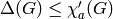 ,
,
 being the maximum degree of , which is given
by the first of the two constraints. Indeed, it is conjectured
that
being the maximum degree of , which is given
by the first of the two constraints. Indeed, it is conjectured
that  .
.
INPUT:
hex_colors (boolean)
- If hex_colors = True, the function returns a dictionary associating to each color a list of edges (meant as an argument to the edge_colors keyword of the plot method).
- If hex_colors = False (default value), returns a list of graphs corresponding to each color class.
value_only (boolean)
- If value_only = True, only returns the acyclic chromatic index as an integer value
- If value_only = False, returns the color classes according to the value of hex_colors
k (integer) – the number of colors to use.
- If k>0, computes an acyclic edge coloring using
colors.
- If k=0 (default), computes a coloring of
colors, which is the conjectured general bound.
- If k=None, computes a decomposition using the least possible number of colors.
**kwds – arguments to be passed down to the solve function of MixedIntegerLinearProgram. See the documentation of MixedIntegerLinearProgram.solve for more informations.
ALGORITHM:
Linear Programming
EXAMPLE:
The complete graph on 8 vertices can not be acyclically
edge-colored with less  colors, but it can be
colored with
colors, but it can be
colored with  :
:
sage: from sage.graphs.graph_coloring import acyclic_edge_coloring
sage: g = graphs.CompleteGraph(8)
sage: colors = acyclic_edge_coloring(g)
Each color class is of course a matching
sage: all([max(gg.degree())<=1 for gg in colors])
True
These matchings being a partition of the edge set:
sage: all([ any([gg.has_edge(e) for gg in colors]) for e in g.edges(labels = False)])
True
Besides, the union of any two of them is a forest
sage: all([g1.union(g2).is_forest() for g1 in colors for g2 in colors])
True
If one wants to acyclically color a cycle on  vertices,
at least 3 colors will be necessary. The function raises
an exception when asked to color it with only 2:
vertices,
at least 3 colors will be necessary. The function raises
an exception when asked to color it with only 2:
sage: g = graphs.CycleGraph(4)
sage: acyclic_edge_coloring(g, k=2)
...
ValueError: This graph can not be colored with the given number of colors.
The optimal coloring give us  classes:
sage: colors = acyclic_edge_coloring(g, k=None)
sage: len(colors)
3
Computes all  -colorings of the graph by casting the graph
coloring problem into an exact cover problem, and passing this
into an implementation of the Dancing Links algorithm described
by Knuth (who attributes the idea to Hitotumatu and Noshita).
-colorings of the graph by casting the graph
coloring problem into an exact cover problem, and passing this
into an implementation of the Dancing Links algorithm described
by Knuth (who attributes the idea to Hitotumatu and Noshita).
The construction works as follows. Columns:
 columns correspond to a vertex – a
  in this
column indicates that that vertex has a color. columns, we add
in this
column indicates that that vertex has a color. columns, we add  columns – a in
these columns indicate that a particular edge is
incident to a vertex with a certain color.
columns – a in
these columns indicate that a particular edge is
incident to a vertex with a certain color.Rows:
rows; one for each color  . Place
a in the column corresponding to the vertex, and a
in the appropriate column for each edge incident to the
vertex, indicating that that edge is incident to the
color .
. Place
a in the column corresponding to the vertex, and a
in the appropriate column for each edge incident to the
vertex, indicating that that edge is incident to the
color . , the above construction cannot be exactly covered
since each edge will be incident to only two vertices
(and hence two colors) - so we add rows, each one
containing a for each of the columns. These
get added to the cover solutions “for free” during the
backtracking.
, the above construction cannot be exactly covered
since each edge will be incident to only two vertices
(and hence two colors) - so we add rows, each one
containing a for each of the columns. These
get added to the cover solutions “for free” during the
backtracking.Note that this construction results in  entries in the matrix. The Dancing Links algorithm uses a
sparse representation, so if the graph is simple,
entries in the matrix. The Dancing Links algorithm uses a
sparse representation, so if the graph is simple,  and
and  , this construction runs in
  time.
Back-conversion to a coloring solution is a simple scan of the
solutions, which will contain
time.
Back-conversion to a coloring solution is a simple scan of the
solutions, which will contain 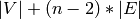 entries, so
runs in time also. For most graphs, the conversion
will be much faster – for example, a planar graph will be
transformed for -coloring in linear time since
entries, so
runs in time also. For most graphs, the conversion
will be much faster – for example, a planar graph will be
transformed for -coloring in linear time since  .
.
REFERENCES:
http://www-cs-staff.stanford.edu/~uno/papers/dancing-color.ps.gz
EXAMPLES:
sage: from sage.graphs.graph_coloring import all_graph_colorings
sage: G = Graph({0:[1,2,3],1:[2]})
sage: n = 0
sage: for C in all_graph_colorings(G,3):
...       parts = [C[k] for k in C]
...       for P in parts:
...           l = len(P)
...           for i in range(l):
...               for j in range(i+1,l):
...                   if G.has_edge(P[i],P[j]):
...                       raise RuntimeError, "Coloring Failed."
...       n+=1
sage: print "G has %s 3-colorings."%n
G has 12 3-colorings.
TESTS:
sage: G = Graph({0:[1,2,3],1:[2]})
sage: for C in all_graph_colorings(G,0): print C
sage: for C in all_graph_colorings(G,-1): print C
...
ValueError: n must be non-negative.
Returns the minimal number of colors needed to color the
vertices of the graph .
EXAMPLES:
sage: from sage.graphs.graph_coloring import chromatic_number
sage: G = Graph({0:[1,2,3],1:[2]})
sage: chromatic_number(G)
3

sage: G = graphs.PetersenGraph()
sage: G.chromatic_number()
3
Properly colors the edges of a graph. See the URL http://en.wikipedia.org/wiki/Edge_coloring for further details on edge coloring.
INPUT:
 -edge-coloring,
where
-edge-coloring,
where  is equal to the maximum degree in the graph.-edge-coloring,
where is equal to the maximum degree in the graph. If
impossible, tries to find and returns a -edge-coloring.
This implies that value_only=False.
is equal to the maximum degree in the graph.-edge-coloring,
where is equal to the maximum degree in the graph. If
impossible, tries to find and returns a -edge-coloring.
This implies that value_only=False. -complete
problem, this function may take some time depending on the graph. Use
log to define the level of verbosity you wantfrom the linear
program solver. By default log=0, meaning that there will be no
message printed by the solver.
-complete
problem, this function may take some time depending on the graph. Use
log to define the level of verbosity you wantfrom the linear
program solver. By default log=0, meaning that there will be no
message printed by the solver.OUTPUT:
In the following, is equal to the maximum degree in the graph
g.
matchings. or to .Note
In a few cases, it is possible to find very quickly the chromatic index of a graph, while it remains a tedious job to compute a corresponding coloring. For this reason, value_only = True can sometimes be much faster, and it is a bad idea to compute the whole coloring if you do not need it !
EXAMPLE:
sage: from sage.graphs.graph_coloring import edge_coloring
sage: g = graphs.PetersenGraph()
sage: edge_coloring(g, value_only=True)
4
Complete graphs are colored using the linear-time round-robin coloring:
sage: from sage.graphs.graph_coloring import edge_coloring
sage: len(edge_coloring(graphs.CompleteGraph(20)))
19
Given a graph, and optionally a natural number , returns
the first coloring we find with at least colors.
INPUT:
EXAMPLES:
sage: from sage.graphs.graph_coloring import first_coloring
sage: G = Graph({0: [1, 2, 3], 1: [2]})
sage: first_coloring(G, 3)
[[1, 3], [0], [2]]
Computes the linear arboricity of the given graph.
The linear arboricity of a graph is the least
number  such that the edges of can be
partitioned into linear forests (i.e. into forests
of paths).
such that the edges of can be
partitioned into linear forests (i.e. into forests
of paths).
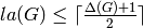
Obviously, 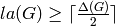 .
.
It is conjectured in [Aki80] that
 .
.
INPUT:
hex_colors (boolean)
- If hex_colors = True, the function returns a dictionary associating to each color a list of edges (meant as an argument to the edge_colors keyword of the plot method).
- If hex_colors = False (default value), returns a list of graphs corresponding to each color class.
value_only (boolean)
- If value_only = True, only returns the linear arboricity as an integer value.
- If value_only = False, returns the color classes according to the value of hex_colors
k (integer) – the number of colors to use.
- If 0, computes a decomposition of
forests of paths
- If 1 (default), computes a decomposition of
colors, which is the conjectured general bound.
- If k=None, computes a decomposition using the least possible number of colors.
**kwds – arguments to be passed down to the solve function of MixedIntegerLinearProgram. See the documentation of MixedIntegerLinearProgram.solve for more informations.
ALGORITHM:
Linear Programming
COMPLEXITY:
NP-Hard
EXAMPLE:
Obviously, a square grid has a linear arboricity of 2, as the set of horizontal lines and the set of vertical lines are an admissible partition:
sage: from sage.graphs.graph_coloring import linear_arboricity
sage: g = graphs.GridGraph([4,4])
sage: g1,g2 = linear_arboricity(g, k=0)
Each graph is of course a forest:
sage: g1.is_forest() and g2.is_forest()
True
Of maximum degree 2:
sage: max(g1.degree()) <= 2 and max(g2.degree()) <= 2
True
Which constitutes a partition of the whole edge set:
sage: all([g1.has_edge(e) or g2.has_edge(e) for e in g.edges(labels = None)])
True
REFERENCES:
| [Aki80] | Akiyama, J. and Exoo, G. and Harary, F. Covering and packing in graphs. III: Cyclic and acyclic invariants Mathematical Institute of the Slovak Academy of Sciences Mathematica Slovaca vol30, n4, pages 405–417, 1980 |
Given a graph and a natural number , returns the number of
-colorings of the graph.
EXAMPLES:
sage: from sage.graphs.graph_coloring import number_of_n_colorings
sage: G = Graph({0:[1,2,3],1:[2]})
sage: number_of_n_colorings(G,3)
12
Returns the number of -colorings of the graph for from
 to .
to .
EXAMPLES:
sage: from sage.graphs.graph_coloring import numbers_of_colorings
sage: G = Graph({0:[1,2,3],1:[2]})
sage: numbers_of_colorings(G)
[0, 0, 0, 12, 72]
Computes a round-robin coloring of the complete graph on vertices.
A round-robin coloring of the complete graph on  vertices
(
vertices
(![V = [0, \dots, 2n - 1]](../../_images/math/e306472f252bab94250ed6188d3928d396311701.png) ) is a proper coloring of its edges such that
the edges with color are all the
) is a proper coloring of its edges such that
the edges with color are all the  plus the
edge
plus the
edge  .
.
If is odd, one obtain a round-robin coloring of the complete graph
through the round-robin coloring of the graph with  vertices.
INPUT:
OUTPUT:
EXAMPLES:
sage: from sage.graphs.graph_coloring import round_robin
sage: round_robin(3).edges()
[(0, 1, 2), (0, 2, 1), (1, 2, 0)]
sage: round_robin(4).edges()
[(0, 1, 2), (0, 2, 1), (0, 3, 0), (1, 2, 0), (1, 3, 1), (2, 3, 2)]
For higher orders, the coloring is still proper and uses the expected number of colors.
sage: g = round_robin(9)
sage: sum([Set([e[2] for e in g.edges_incident(v)]).cardinality() for v in g]) == 2*g.size()
True
sage: Set([e[2] for e in g.edge_iterator()]).cardinality()
9
sage: g = round_robin(10)
sage: sum([Set([e[2] for e in g.edges_incident(v)]).cardinality() for v in g]) == 2*g.size()
True
sage: Set([e[2] for e in g.edge_iterator()]).cardinality()
9
Computes the chromatic number of the given graph or tests its
-colorability. See http://en.wikipedia.org/wiki/Graph_coloring for
further details on graph coloring.
INPUT:
-colorable.
The function returns a partition of the vertex set in independent
sets if possible and False otherwise.-complete
problem, this function may take some time depending on the graph.
Use log to define the level of verbosity you want from the
linear program solver. By default log=0, meaning that there will
be no message printed by the solver.OUTPUT:
-colorable, and a partition of the vertex set into
independent sets otherwise.-colorable, and return True or False accordingly.EXAMPLE:
sage: from sage.graphs.graph_coloring import vertex_coloring
sage: g = graphs.PetersenGraph()
sage: vertex_coloring(g, value_only=True)
3