Cvxopt

Cvxopt provides many routines for solving convex optimization problems such as linear and quadratic programming packages. It also has a very nice sparse matrix library that provides an interface to umfpack (the same sparse matrix solver that matlab uses), it also has a nice interface to lapack. For more details on cvxopt please refer to its documentation at http://abel.ee.ucla.edu/cvxopt/documentation/users-guide/

Sparse matrices are represented in triplet notation that is as a list of nonzero values, row indices and column indices. This is internally converted to compressed sparse column format. So for example we would enter the matrix

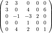
by

sage: import numpy
sage: from cvxopt.base import spmatrix
sage: from cvxopt.base import matrix as m
sage: from cvxopt import umfpack
sage: Integer=int
sage: V = [2,3, 3,-1,4, 4,-3,1,2, 2, 6,1]
sage: I = [0,1, 0, 2,4, 1, 2,3,4, 2, 1,4]
sage: J = [0,0, 1, 1,1, 2, 2,2,2, 3, 4,4]
sage: A = spmatrix(V,I,J)

To solve an equation , with , we could do the following.

sage: B = numpy.array([1.0]*5)
sage: B.shape=(5,1)
sage: print(B)
[[ 1.]
 [ 1.]
 [ 1.]
 [ 1.]
 [ 1.]]
sage: print(A)
SIZE: (5,5)
    (0, 0)  2.0000e+00
    (1, 0)  3.0000e+00
    (0, 1)  3.0000e+00
    (2, 1) -1.0000e+00
    (4, 1)  4.0000e+00
    (1, 2)  4.0000e+00
    (2, 2) -3.0000e+00
    (3, 2)  1.0000e+00
    (4, 2)  2.0000e+00
    (2, 3)  2.0000e+00
    (1, 4)  6.0000e+00
    (4, 4)  1.0000e+00
sage: C=m(B)
sage: umfpack.linsolve(A,C)
sage: print(C)
   5.7895e-01
   -5.2632e-02
   1.0000e+00
   1.9737e+00
   -7.8947e-01

Note the solution is stored in afterward. also note the m(B), this turns our numpy array into a format cvxopt understands. You can directly create a cvxopt matrix using cvxopt’s own matrix command, but I personally find numpy arrays nicer. Also note we explicitly set the shape of the numpy array to make it clear it was a column vector.

We could compute the approximate minimum degree ordering by doing

sage: RealNumber=float
sage: Integer=int
sage: from cvxopt.base import spmatrix
sage: from cvxopt import amd
sage: A=spmatrix([10,3,5,-2,5,2],[0,2,1,2,2,3],[0,0,1,1,2,3])
sage: P=amd.order(A)
sage: print(P)
1
0
2
3

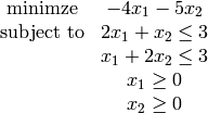
For a simple linear programming example, if we want to solve

sage: RealNumber=float
sage: Integer=int
sage: from cvxopt.base import matrix as m
sage: from cvxopt import solvers
sage: c = m([-4., -5.])
sage: G = m([[2., 1., -1., 0.], [1., 2., 0., -1.]])
sage: h = m([3., 3., 0., 0.])
sage: sol = solvers.lp(c,G,h) #random
     pcost       dcost       gap    pres   dres   k/t
 0: -8.1000e+00 -1.8300e+01  4e+00  0e+00  8e-01  1e+00
 1: -8.8055e+00 -9.4357e+00  2e-01  1e-16  4e-02  3e-02
 2: -8.9981e+00 -9.0049e+00  2e-03  1e-16  5e-04  4e-04
 3: -9.0000e+00 -9.0000e+00  2e-05  3e-16  5e-06  4e-06
 4: -9.0000e+00 -9.0000e+00  2e-07  1e-16  5e-08  4e-08

sage: print sol['x']      # ... below since can get -00 or +00 depending on architecture
   1.0000e...00
   1.0000e+00