Plotting

Sage can plot using matplotlib, openmath, gnuplot, or surf but only matplotlib and openmath are included with Sage in the standard distribution. For surf examples, see Plotting surfaces.

Plotting in Sage can be done in many different ways. You can plot a function (in 2 or 3 dimensions) or a set of points (in 2-D only) via gnuplot, you can plot a solution to a differential equation via Maxima (which in turn calls gnuplot or openmath), or you can use Singular’s interface with the plotting package surf (which does not come with Sage). gnuplot does not have an implicit plotting command, so if you want to plot a curve or surface using an implicit plot, it is best to use the Singular’s interface to surf, as described in chapter ch:AG, Algebraic geometry.

Plotting functions in 2D

The default plotting method in uses the excellent matplotlib package.

To view any of these, type P.save("<path>/myplot.png") and then open it in a graphics viewer such as gimp.

You can plot piecewise-defined functions:

sage: f1 = lambda x:1
sage: f2 = lambda x:1-x
sage: f3 = lambda x:exp(x)
sage: f4 = lambda x:sin(2*x)
sage: f = Piecewise([[(0,1),f1],[(1,2),f2],[(2,3),f3],[(3,10),f4]])
sage: f.plot()

Other function plots can be produced as well:

A red plot of the Jacobi elliptic function , (do not type the ...:

sage: L = [(i/100.0, maxima.eval('jacobi_sn (%s/100.0,2.0)'%i))\
...   for i in range(-300,300)]
sage: show(line(L, rgbcolor=(3/4,1/4,1/8)))

A red plot of -Bessel function , :

sage: L = [(i/10.0, maxima.eval('bessel_j (2,%s/10.0)'%i)) for i in range(100)]
sage: show(line(L, rgbcolor=(3/4,1/4,5/8)))

A purple plot of the Riemann zeta function , :

sage: I = CDF.0
sage: show(line([zeta(1/2 + k*I/6) for k in range(180)], rgbcolor=(3/4,1/2,5/8)))

Plotting curves

To plot a curve in Sage, you can use Singular and surf (http://surf.sourceforge.net/, also available as an experimental package) or use matplotlib (included with Sage).

matplotlib

Here are several examples. To view them, type p.save("<path>/my_plot.png") (where <path> is a directory path which you have write permissions to where you want to save the plot) and view it in a viewer (such as GIMP).

A blue conchoid of Nicomedes:

sage: L = [[1+5*cos(pi/2+pi*i/100), tan(pi/2+pi*i/100)*\
...   (1+5*cos(pi/2+pi*i/100))] for i in range(1,100)]
sage: line(L, rgbcolor=(1/4,1/8,3/4))

A blue hypotrochoid (3 leaves):

sage: n = 4; h = 3; b = 2
sage: L = [[n*cos(pi*i/100)+h*cos((n/b)*pi*i/100),\
...   n*sin(pi*i/100)-h*sin((n/b)*pi*i/100)] for i in range(200)]
sage: line(L, rgbcolor=(1/4,1/4,3/4))

A blue hypotrochoid (4 leaves):

sage: n = 6; h = 5; b = 2
sage: L = [[n*cos(pi*i/100)+h*cos((n/b)*pi*i/100),\
...   n*sin(pi*i/100)-h*sin((n/b)*pi*i/100)] for i in range(200)]
sage: line(L, rgbcolor=(1/4,1/4,3/4))

A red limaçon of Pascal:

sage: L = [[sin(pi*i/100)+sin(pi*i/50),-(1+cos(pi*i/100)+cos(pi*i/50))]\
...   for i in range(-100,101)]
sage: line(L, rgbcolor=(1,1/4,1/2))

A light green trisectrix of Maclaurin:

sage: L = [[2*(1-4*cos(-pi/2+pi*i/100)^2),10*tan(-pi/2+pi*i/100)*\
...   (1-4*cos(-pi/2+pi*i/100)^2)] for i in range(1,100)]
sage: line(L, rgbcolor=(1/4,1,1/8))

A green lemniscate of Bernoulli (we omit i==100 since that would give a 0 division error):

sage: v = [(1/cos(-pi/2+pi*i/100), tan(-pi/2+pi*i/100)) for i in range(1,200) if i!=100 ]
sage: L = [(a/(a^2+b^2), b/(a^2+b^2)) for a,b in v]
sage: line(L, rgbcolor=(1/4,3/4,1/8))

surf

In particular, since surf is only available on a UNIX type OS (and is not included with Sage), plotting using the commands below in Sage is only available on such an OS. Incidentally, surf is included with several popular Linux distributions.

sage: s = singular.eval
sage: s('LIB "surf.lib";')
...
sage: s("ring rr0 = 0,(x1,x2),dp;")
''
sage: s("ideal I = x1^3 - x2^2;")
''
sage: s("plot(I);")
...

Press q with the surf window active to exit from surf and return to Sage.

You can save this plot as a surf script. In the surf window which pops up, just choose file, save as, etc.. (Type q or select file, quit, to close the window.)

The plot produced is omitted but the gentle reader is encouraged to try it out.

openmath

Openmath is a TCL/Tk GUI plotting program written by W. Schelter.

The following command plots the function

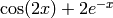
sage: maxima.plot2d('cos(2*x) + 2*exp(-x)','[x,0,1]',\
...   '[plot_format,openmath]')  # optional -- pops up a window.

(Mac OS X users: Note that these openmath commands were run in a session of started in an xterm shell, not using the standard Mac Terminal application.)

sage: maxima.eval('load("plotdf");')
'".../local/share/maxima/.../share/dynamics/plotdf.lisp"'
sage: maxima.eval('plotdf(x+y,[trajectory_at,2,-0.1]); ') #optional

This plots a direction field (the plotdf Maxima package was also written by W. Schelter.)

A 2D plot of several functions:

sage: maxima.plot2d('[x,x^2,x^3]','[x,-1,1]','[plot_format,openmath]') #optional

Openmath also does 3D plots of surfaces of the form , as and range over a rectangle. For example, here is a “live” 3D plot which you can move with your mouse:

sage: maxima.plot3d ("sin(x^2 + y^2)", "[x, -3, 3]", "[y, -3, 3]",\
...   '[plot_format, openmath]') #optional

By rotating this suitably, you can view the contour plot.

Tachyon 3D plotting

The ray-tracing package Tachyon is distributed with Sage. The 3D plots look very nice but tend to take a bit more setting up. Here is an example of a parametric space curve:

sage: f = lambda t: (t,t^2,t^3)
sage: t = Tachyon(camera_center=(5,0,4))
sage: t.texture('t')
sage: t.light((-20,-20,40), 0.2, (1,1,1))
sage: t.parametric_plot(f,-5,5,'t',min_depth=6)

Type t.show() to view this.

Other examples are in the Reference Manual.

gnuplot

You must have gnuplot installed to run these commands. This is an “experimental package” which, if it isn’t installed already on your machine, can be (hopefully!) installed by typing ./sage -i gnuplot-4.0.0 on the command line in the Sage home directory.

First, here’s way to plot a function: {plot!a function}

sage: maxima.plot2d('sin(x)','[x,-5,5]')
sage: opts = '[gnuplot_term, ps], [gnuplot_out_file, "sin-plot.eps"]'
sage: maxima.plot2d('sin(x)','[x,-5,5]',opts)
sage: opts = '[gnuplot_term, ps], [gnuplot_out_file, "/tmp/sin-plot.eps"]'
sage: maxima.plot2d('sin(x)','[x,-5,5]',opts)

The eps file is saved by default to the current directory but you may specify a path if you prefer.

Here is an example of a plot of a parametric curve in the plane:

sage: maxima.plot2d_parametric(["sin(t)","cos(t)"], "t",[-3.1,3.1])
sage: opts = '[gnuplot_preamble, "set nokey"], [gnuplot_term, ps],\
...   [gnuplot_out_file, "circle-plot.eps"]'
sage: maxima.plot2d_parametric(["sin(t)","cos(t)"], "t", [-3.1,3.1], options=opts)

Here is an example of a plot of a parametric surface in 3-space: {plot!a parametric surface}

sage: maxima.plot3d_parametric(["v*sin(u)","v*cos(u)","v"], ["u","v"],\
...   [-3.2,3.2],[0,3])      # optional -- pops up a window.
sage: opts = '[gnuplot_term, ps], [gnuplot_out_file, "sin-cos-plot.eps"]'
sage: maxima.plot3d_parametric(["v*sin(u)","v*cos(u)","v"], ["u","v"],\
...   [-3.2,3.2],[0,3],opts)     # optional -- pops up a window.

To illustrate how to pass gnuplot options in , here is an example of a plot of a set of points involving the Riemann zeta function (computed using Pari but plotted using Maxima and Gnuplot): {plot!points} {Riemann zeta function}

sage: zeta_ptsx = [ (pari(1/2 + i*I/10).zeta().real()).precision(1)\
...   for i in range (70,150)]
sage: zeta_ptsy = [ (pari(1/2 + i*I/10).zeta().imag()).precision(1)\
...   for i in range (70,150)]
sage: maxima.plot_list(zeta_ptsx, zeta_ptsy)  # optional -- pops up a window.
sage: opts='[gnuplot_preamble, "set nokey"], [gnuplot_term, ps],\
...   [gnuplot_out_file, "zeta.eps"]'
sage: maxima.plot_list(zeta_ptsx, zeta_ptsy, opts) # optional -- pops up a window.

Plotting surfaces

To plot a surface in is no different that to plot a curve, though the syntax is slightly different. In particular, you need to have surf loaded. {plot!surface using surf}

sage: singular.eval('ring rr1 = 0,(x,y,z),dp;')
''
sage: singular.eval('ideal I(1) = 2x2-1/2x3 +1-y+1;')
''
sage: singular.eval('plot(I(1));')
...