


: Bibliography
: One-dimensional Shape Memory Alloy
: One-dimensional Shape Memory Alloy
In this paper we are concerned with the global existence and uniqueness of
a solution to a one-dimensional model of thermomechanical evolution of
shape memory alloys. First, the following two differential equations are
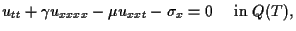
derived from the conservation laws of linear momentum and energy:
|
(1.1) |
|
|
 |
|
(1.2) |
|
|
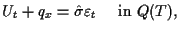 |
where  denotes the displacement,
 is the
strain,
is the
strain,  is the stress,
 is the internal energy,
  is the heat flux and
 is a positive constant.
Here, we refer Brokate-Sprekels
[4, Section 5] and Pawlow [10]
for the physical background of these laws.
Now, we use the classical Fourier law and an elementary approximation
is a positive constant.
Here, we refer Brokate-Sprekels
[4, Section 5] and Pawlow [10]
for the physical background of these laws.
Now, we use the classical Fourier law and an elementary approximation
 where
where
 is the temperature field.
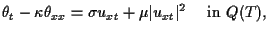
Therefore, (1.2) can be written by
is the temperature field.
Therefore, (1.2) can be written by
|
(1.3) |
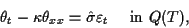 |
where  is a positive constant depending on the specific heat and
the heat conductivity.
By some mathematical reasons
we assume that there are interior frictions in the form
of viscous stresses in the material. Then we can apply
Hooke's-like law so that we have
is a positive constant depending on the specific heat and
the heat conductivity.
By some mathematical reasons
we assume that there are interior frictions in the form
of viscous stresses in the material. Then we can apply
Hooke's-like law so that we have
|
(1.4) |
 |
where  is the constant viscosity.
The above composition of the stress was investigated by many mathematicians
(cf. [9,6,4]).
Falk's model [5] is well known as the system describing the dynamics
of one-dimensional shape memory alloys.
Falk's model is based on the Landau-Devonshire theory. This means that
is the constant viscosity.
The above composition of the stress was investigated by many mathematicians
(cf. [9,6,4]).
Falk's model [5] is well known as the system describing the dynamics
of one-dimensional shape memory alloys.
Falk's model is based on the Landau-Devonshire theory. This means that
 is decided by the derivative of
the Helmholtz energy
is decided by the derivative of
the Helmholtz energy
 , that is,
However, by some experiments we know that
the relationship between the stress and the strain is described by
the hysteresis loop depending on the temperature.
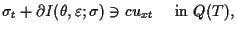
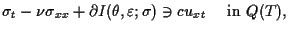
In our previous works [1,2] we have already pointed out that the relationship can be represented by the
ordinary differential equations including the subdifferentials of the
indicator function of the closed interval as follows:
|
(1.5) |
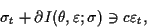 |
where  is a positive constant depending on the hysteresis loops
and
is a positive constant depending on the hysteresis loops
and  is the indicator function of
the closed interval
is the indicator function of
the closed interval
![$[f_a(\theta,\varepsilon), f_d(\theta,\varepsilon)]$](img22.png) for
given continuous functions
for
given continuous functions  and
and  on
on  with
with  on ,
that is,
on ,
that is,
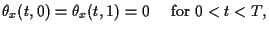
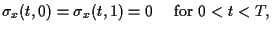
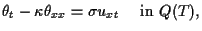
Therefore the following system P P
P
 is derived from (1.1) and (1.3)
 (1.5).
|
(1.6) |
|
|
 |
|
(1.7) |
|
|
 |
|
(1.8) |
|
|
 |
|
(1.9) |
|
|
 |
|
(1.10) |
|
|
 |
|
(1.11) |
|
|
 |
|
(1.12) |
|
|
 |
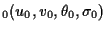
where  ,
,  ,
,  and
and  are given initial functions.
Our formulation does not require the monotonicity for and ,
but needs the boundedness of and on .
Moreover, it can cover the special case where
which gives a Falk-type model with bounded.
The main purpose of this paper is to give the existence and uniqueness theorem
for P .
In [1] we have already proved the wellposedness for P with
(1.13) and (1.14) instead of (1.7) and
(1.8), respectively.
.
In [1] we have already proved the wellposedness for P with
(1.13) and (1.14) instead of (1.7) and
(1.8), respectively.
|
(1.13) |
|
|
 |
|
(1.14) |
|
|
 |
where  is a positive constant.
Also, in [2] we studied P with (1.14) instead of
(1.8), which is denoted by
P
is a positive constant.
Also, in [2] we studied P with (1.14) instead of
(1.8), which is denoted by
P P
P
 for .
for .
In this paper we refer the book [3] and
[7] for the theory on
maximal monotone operators and subdifferentials of convex functions in
a Hilbert space.
: Bibliography
: One-dimensional Shape Memory Alloy
: One-dimensional Shape Memory Alloy
Nobuki Takayama
Heisei 16-1-21.