Introduction

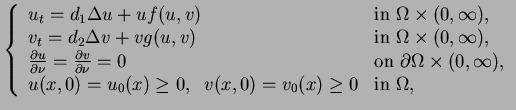
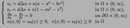
In this paper we study the global behavior of solutions to the reaction-diffusion system :

$$\left\{ \begin{array}{ll} u_t = d_1 \ensuremath{\Delta}u + uf(u,v... ...u_0 (x)\ge 0, \;\; v(x,0)=v_0 (x)\ge 0 & \mbox{in $\Omega$}, \end{array}\right.$$ (1.1)

where $\Omega$ is a bounded smooth domain in $\mathbb{R}^n$ and $\nu$ is the outward unit normal vector to $\partial \Omega$. The initial functions $u_0(x)$, $v_0(x)$ are not identically zero, and the functions $f(u,v)$ and $g(u,v)$ are of class $C^1(Q)$ where

$$Q=\{(u,v)\in \mathbb{R}^2\vert u\ge 0, v\ge 0\}. \vspace{-0.1cm}$$

For $f(u,v)$ and $g(u,v)$ we will consider the following two cases of competition type which make (1.1) a competition-diffusion system :

$(\ensuremath{\alpha})$

$f(u,v)=a_1 -b_1 u -c_1 v, \;\;\;\;\;\; g(u,v)=a_2 -b_2 u-c_2 v$,

$(\beta)$

$f(u,v)=a_1 -b_1 u^2 -c_1 v^2, \;\;\; g(u,v)=a_2 -b_2 u^2-c_2 v^2$.

In the system (1.1) $u$ and $v$ are nonnegative functions which represent the population densities of two competing species. $d_1$ and $d_2$ are the diffusion rates of the two species, respectively. $a_1$ and $a_2$ denote the intrinsic growth rates, $b_1$ and $c_2$ account for intra-specific competitions, $b_2$ and $c_1$ are the coefficients for inter-specific competitions. For details on the backgrounds of this model, we refer the reader to [6].

Remark. The linear functions for $f(u,v)$ and $g(u,v)$ as in ${\bf (\ensuremath{\alpha})}$ are often used in the classical competition-diffusion systems. Though the quadratic functions for $f(u,v)$ and $g(u,v)$ as in ${\bf (\beta)}$ may not be used commonly, they make the system (1.1) the gradient system of an energy functional (after simple scalings) which helps one to analyze the system (1.1) more clearly. And, in the course of this paper it will be shown that the system (1.1) with ${\bf (\beta)}$ has similar properties as the system with ${\bf (\ensuremath{\alpha})}$.

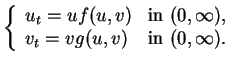
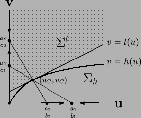
The global behavior of solutions to the system (1.1) is related to that of its kinetic system which is the following system of ordinary differential equations :

$$\left\{ \begin{array}{ll} u_t = uf(u,v)& \mbox{in }(0,\infty), \\ v_t = vg(u,v)& \mbox{in }(0,\infty). \end{array}\right.$$ (1.2)

Clearly $Q$ is positively invariant for the flow of (1.2). The equilibria of the kinetic system (1.2) in $Q$ consist of four points $(u_A,0)$, $(0,v_B)$, $(u_C, v_C)$ and $(0,0)$, where $u_A$, $v_B$, $u_C$ and $v_C$ are positive constants in both cases $\bf {(\ensuremath {\alpha })}$ and $\bf {(\beta )}$ of the functions $f(u,v)$ and $g(u,v)$. Throughout this paper we impose the following strong competition conditions on the coefficients in $f(u,v)$ and $g(u,v)$ :

$$\frac{b_1}{b_2}<\frac{a_1}{a_2}<\frac{c_1}{c_2}. \vspace{-0.1cm}$$ (1.3)

We note that the condition (1.3) assures that $(0,0)$ is unstable, $(u_A,0)$, $(0,v_B)$ are stable, and $(u_C, v_C)$ is a saddle point for (1.2). The flows of the kinetic system (1.2) under the condition (1.3) are shown in Figure (1).

Figure 1: Flows of (1.2) with competitions as in $\bf{(\ensuremath{\alpha})}$ and in $\bf{(\beta)}$.

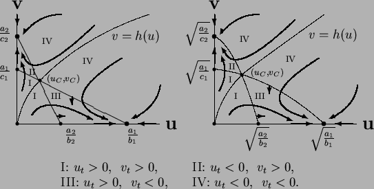
For the general properties of separatrix $h(u)$ of the kinetic system (1.2) which is illustrated in Figure 1 we refer the reader to the result due to Iida et al. [2] which is stated in Proposition 1.1 in the following. The reader may also refer to Hirsch and Smale [1], Ninomiya [5] for the properties of separatrices.

Proposition 1.1   Suppose for the system (1.2) that $f(u,v)$ and $g(u,v)$ are as in either $\bf {(\ensuremath {\alpha })}$ or $\bf {(\beta )}$. Then there exists a monotone function $h(u)$ defined on $[0,u_{\infty})$ with $u_{\infty}\in(u_C,\infty]$ such that

$W_A=\{(u,v)\in Q\vert v<h(u)\}$ is the basin of attraction for $(u_A,0)$,

$W_B=\{(u,v)\in Q\vert v>h(u)\}$ is the basin of attraction for $(0,u_B)$,

$\Gamma =\{(u,v)\in Q\vert v=h(u)\}$ is the separatrix.

Moreover $h(u)$ satisfies

(i)

$h(0)=0$,

(ii)

$h(u_C)=v_C$,

(iii)

$\lim_{u\rightarrow u_{\infty}}h(u)=\infty$ if $u_{\infty}<\infty$,

(iv)

$h'(u)>0$ on $(0,u_{\infty})$,

(v)

$u f(u,h(u))h'(u)=h(u)g(u,h(u))$ on $(0,u_{\infty})$,

(vi)

$f(u,h(u))g(u,h(u))>0$ on $(0,u_C)\cup(u_C,u_{\infty})$.

Iida et al. [2] assumed in addition to the strong-competition condition (1.3) that $\frac{a_1}{a_2}\ge 1$ which means that the species $u$ is superior to the other species $v$ in the competition sense, and they showed that the separatrix of the kinetic system (1.2) with linear competitions as in $(\ensuremath{\alpha})$ is concave, i.e. $h''\le 0$. Also assuming that $d_1=d_2$ they proved that the region under the concave separatrix is a domain of attraction for the equilibrium point $(u_A,0)=(\frac{a_1}{b_1},0)$ in the phase plane for the competition-diffusion system (1.1) with linear competitions as in $(\ensuremath{\alpha})$. Their result means in Figure 2 that if the initial state $(u_0(x), v_0(x))$ is chosen in the region $\Sigma_h$ then the solution $(u(x,t), v(x,t))$ converges to $(u_A,0)$, that is, only the superior species $u$ survives and the inferior species $v$ is wiped out eventually. In this paper we are interested in finding the initial states for which the inferior species $v$ survives and the superior species $u$ dies out at the end. First we consider the same situation as Iida et al. [2] and prove that the region $\Sigma ^l$ above the concave separatrix in Figure 2 is a domain of attraction of the equilibrium point $(0,u_B)=(0,\frac{a_2}{c_2})$. We later consider the quadratic competitions as in $(\beta)$ for the competition-diffusion system (1.1) with $d_1=d_2$ to show that the region $\Sigma ^l$ above the separatrix in Figure 3 is a domain of attraction of the equilibrium point $(0, u_B)=(0,\sqrt{\frac{a_2}{c_2}})$.

Figure: The set $\Sigma ^l$ for the system (1.1) with linear competitions.

Figure: The set $\Sigma ^l$ for the system (1.1) with quadratic competitions.

In order to state our main results we introduce the notation which will be used throughout this paper, and reduce the system (1.1) with $d_1=d_2$ and the strong competition condition (1.3) to a simpler form.

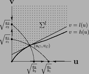
Notation. We set $\Sigma^k :=\{ (u,v) \in Q \vert \; u \ge 0,\;\; v > k(u) \}$, where $k(u)$ is a strictly increasing $C^2$-function with $k(0) \ge 0$. We denote $v=l(u)$ the tangent line of $v=h(u)$ at the unstable constant equilibrium $(u_C, v_C)$ in the phase plane.

The competition-diffusion system (1.1) with $d_1=d_2=d$ and linear competitions as in $\bf {(\ensuremath {\alpha })}$ is reduced to the following system :

$$\left\{ \begin{array}{ll} u_t = d \ensuremath{\Delta}u + u(a-u-bv... ... = u_0 (x)\ge 0, \;\; v(x,0)=v_0 (x)\ge 0 & \mbox{in }\Omega \end{array}\right.$$ (1.4)

by the change of variables $\tau=a_2 t$, $\tilde u=\frac{b_1}{a_2}u$ and $\tilde v=\frac{c_2}{a_2}v$, and then using the variables $t$, $u$ and $v$ instead of $\tau$, $\tilde u$ and $\tilde v$. The equilibria in $Q$ for the kinetic system of (1.4) consist of four points, $(u_A,0)=(a,0)$, $(0,v_B)=(0,1)$, $(u_C, v_C)=(\frac{b-a}{bc-1},\frac{ac-1}{bc-1})$, and $(0,0)$.

The competition-diffusion systems (1.1) with $d_1=d_2=d$ and quadratic competitions as in $\bf {(\beta )}$ is reduced to the following system :

$$\left\{ \begin{array}{ll} u_t = d \ensuremath{\Delta}u + u(a-u^2-... ... = u_0 (x)\ge 0, \;\; v(x,0)=v_0 (x)\ge 0 & \mbox{in }\Omega \end{array}\right.$$ (1.5)

by the change of variables $\tau=a_2 t$, $\tilde u=\sqrt{\frac{b_1}{a_2}}u$ and $\tilde v=\sqrt{\frac{c_2}{a_2}}v$, and then using the variables $t$, $u$ and $v$ instead of $\tau$, $\tilde u$ and $\tilde v$. The equilibria in $Q$ for the kinetic system of (1.5) consist of four points, $(u_A,0)=(\sqrt a,0)$, $(0,v_B)=(0,1)$, $(u_C, v_C)=(\sqrt{\frac{b-a}{bc-1}},\sqrt{\frac{ac-1}{bc-1}})$, and $(0,0)$.

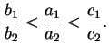
For both systems (1.4) and (1.5) the strong competition condition (1.3) is reduced to

$$\frac 1 c < a < b .$$ (1.6)

Now we present our main results in the following theorems.

Theorem 1.1   Let $\frac 1 c < a < b$, $a\ge 1$, and $(u_0 (x),v_0 (x))\in \Sigma^l$. Then a solution $(u(x,t), v(x,t))$ of the system (1.4) stays in the set $\Sigma ^l$ and converges to $(0,1)$ uniformly as $t\rightarrow \infty$.

Theorem 1.2   Let $\frac 1 c < a < b$, $a\ge 1$, and $(u_0 (x),v_0 (x))\in \Sigma^l$. Suppose that $h''(u) \le 0$ for $u<u_C$. Then a solution $(u(x,t), v(x,t))$ of the system (1.5) stays in the set $\Sigma ^l$ and converges to $(0,1)$ uniformly as $t\rightarrow \infty$.

Remark. In the proofs of Theorems 1.1 and 1.2 the concavity of the graph of the function $h(u)$ plays an important role. Regarding the system (1.4) the concavity of $h$ is proved by Iida et al. [2] as stated in Proposition 2.1. We prove similar but partial result for the system (1.5) in Proposition 2.2. A sufficient condition on the coefficients $a$, $b$, $c$ to guarantee that $h''(u) \le 0$ for $u<u_C$ is found in Proposition 2.2 (vi).

The properties of separatrix which are needed during the constructions of domains of attraction are studied in Section 2. In Section 3 we obtain the invariance of the set $\overline {\Sigma^l}$ for the flow (1.4) and (1.5). We present lemmas regarding auxiliary functions which are used in the proofs of Theorem 1.1 and Theorem 1.2 in Section 4. The proofs of Theorem 1.1 and Theorem 1.2 are given in Section 5 and 6, respectively.