There is a large literature on the equation (1.1); see [,3,4,,6,,8,9,,,14,16,,17,18,,22,23,,21]
and references therein.
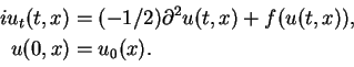
The well-posedness of the Cauchy Problem (1.1) has been
extensively studied,
and the results already obtained are satisfactory
for our study of the asymptotic behavior of the solution.
To put it briefly,
if
![]() , the equation (1.1) is (conditionally)
well-posed in
, the equation (1.1) is (conditionally)
well-posed in ![]() ,
and moreover
,
and moreover
![]() if
if
![]() with
with ![]() .
Here
.
Here
![]() is the free propagator and
is the free propagator and
![]() denotes the weighted
denotes the weighted ![]() -space of order
-space of order ![]() ;
more precisely, see Proposition 2.4 below.
In what follows, we simply call the solution obtained by Proposition
2.4
``the solution to (1.1).''
;
more precisely, see Proposition 2.4 below.
In what follows, we simply call the solution obtained by Proposition
2.4
``the solution to (1.1).''
The asymptotic behavior of the solution to (1.1) is usually
explained in terms of the scattering theory.
When
![]() , the solution is expected to decay by the dispersive
effect of the equation.
Hence we can expect that the nonlinearity in the equation decays
rapidly enough and loses its effect as
, the solution is expected to decay by the dispersive
effect of the equation.
Hence we can expect that the nonlinearity in the equation decays
rapidly enough and loses its effect as
![]() .
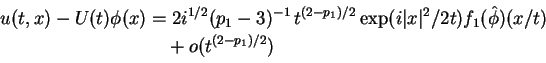
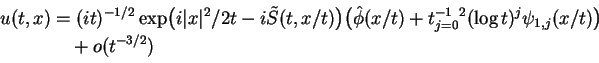
Thus the expected profile of the solution to (1.1) is of the form
.
Thus the expected profile of the solution to (1.1) is of the form
![]() ,
which is a solution to the free Schrödinger equation;
here
,
which is a solution to the free Schrödinger equation;
here ![]() is a suitable function called the scattering state of the solution.
This observation is, however,
correct only in case
is a suitable function called the scattering state of the solution.
This observation is, however,
correct only in case ![]() , namely the short-range case
(on the other hand, the nonlinear term with
, namely the short-range case
(on the other hand, the nonlinear term with ![]() is
called of long-range).
Indeed, the followings are well known [,12,].
is
called of long-range).
Indeed, the followings are well known [,12,].
| (1.4) |
The purpose of this paper is to treat the case ![]() .
The equation (1.1) with
.
The equation (1.1) with ![]() appears various fields of mathematical physics,
and hence it is considered to be important.
Since this case is of long-range, mathematical treatment is more difficult
than short-range case.
Now we state our theorem.
appears various fields of mathematical physics,
and hence it is considered to be important.
Since this case is of long-range, mathematical treatment is more difficult
than short-range case.
Now we state our theorem.
| (1.11) | ||
| (1.12) | ||
| (1.13) |
In the previous paper [24],
one of the authors showed an analogous result for the Hartree equation
which includes the nonlinearity like
![]() .
The treatment of (1.1) is more difficult
than that of the Hartree equation by the following reason.
While the nonlinear term in the Hartree equation can be differentiated
as many times as we like,
the short-range nonlinear perturbation
.
The treatment of (1.1) is more difficult
than that of the Hartree equation by the following reason.
While the nonlinear term in the Hartree equation can be differentiated
as many times as we like,
the short-range nonlinear perturbation ![]() in (1.1) is differentiable
at most
in (1.1) is differentiable
at most ![]() -times because of the singularity at
-times because of the singularity at ![]() .
Thus, in case
.
Thus, in case ![]() is close to
is close to ![]() , we can differentiate the phase
, we can differentiate the phase
![]() only
only
![]() times,
which is not sufficient to prove the theorem as long as we
rely on
times,
which is not sufficient to prove the theorem as long as we
rely on ![]() -theory;
indeed, we would need
-theory;
indeed, we would need ![]() and hence
and hence ![]() .
To avoid this difficulty and prove the theorem for
.
To avoid this difficulty and prove the theorem for ![]() , we state
Proposition 3.2
in terms of the Besov space
, we state
Proposition 3.2
in terms of the Besov space
![]() with
with
![]() ,
, ![]() ,
which is continuously embedded in
,
which is continuously embedded in
![]() .
.
We shall conclude this introduction by giving the notation used in this paper:
![]() is the Fourier transform of
is the Fourier transform of ![]() , and
, and
![]() its inverse.
For
its inverse.
For
![]() ,
,
![]() means the usual
means the usual ![]() -norm;
-norm;
![]() denotes the weighted Lebesgue space;
denotes the weighted Lebesgue space;
![]() denotes the Sobolev space,
denotes the Sobolev space, ![]() is abbreviated to
is abbreviated to ![]() ;
;
![]() denotes the Besov space (see section 2).
denotes the Besov space (see section 2).
![]() ,
,
![]() ,
,
![]() .
.