Finite Dimensional Attractor for one-dimensional Keller-Segel Equations

Koichi Osaki and Atsushi Yagi (Osaka University)

Funkcialaj Ekvacioj, 44 (2001), 441-469

Full Article

Introduction
In this paper, we study the long time behavior of a one-dimensional reaction diffusion system appearing in mathematical biology by using the theory of infinite dimensional dynamical systems.

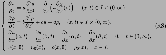
In 1970 Keller and Segel [9] have presented parabolic systems to describe the aggregation process of cellular slime mold by the chemical attraction. The system of a simplified form in the one-dimensional case is written as

$$\left\{\begin{array}{l} \dfrac{\partial u}{\partial t} = a \dfrac... ...\quad \rho(x,0) = \rho_0(x), \quad x \in I. \end{array} \right.\leqno{\rm (KS)}$$

Here, $I = (\alpha, \beta)$ is a bounded open interval. $a, b, c$ and $d$ are positive constants. The unknown functions $u = u(x,t)$ and $\rho = \rho(x,t)$ denote the concentration of amoebae and the concentration of chemical substance, respectively, in $I \times (0, \infty)$. The chemotactic term $- \frac{\partial}{\partial x} (u \frac{\partial \chi}{\partial x}(\rho) )$ indicates that the cells are sensitive to the chemicals and are attracted by them. $\chi(\rho)$ called the sensitivity function is a smooth function of $\rho \in (0, \infty)$ which describes cell's perception and response to the chemical stimulus $\rho$. Several normalized forms have been suggested: $\rho$, $\rho^2$, $\log \rho$, $\frac{\rho}{1 + \rho}$ and $\frac{\rho^2}{1 + \rho^2}$, etc., see [10] and [17]. In view of these forms, we will assume in this paper (except in the last section) that:
($\chi$) $\chi(\rho)$ is a smooth function of $\rho \in (0, \infty)$ and its three derivatives satisfy the estimates

$$\vert \chi^{(i)}(\rho) \vert \le C \Big( \rho + \frac{1}{\rho} \Big)^{r}, \quad 0 < \rho < \infty,\ i = 1, 2, 3$$

with some positive constant $C$ and exponent $r$.
The system (KS) is called the Keller-Segel equations.

In these years the Keller-Segel equations attracted interests of many mathematicians. The local solutions were studied by the second author [23]. It was also suggested in [23] that, in the one-dimensional case, (KS) possesses a global solution and that, in the two-dimensional case, when $\chi(\rho) = k \rho$ ($k$ being a positive constant) is a linear function, (KS) possesses a global solution for any sufficiently small initial function $u_{0}$. Afterward Nagai et al. [13] showed more strongly that the global solution exists if the norm $\Vert u_{0} \Vert _{L^1}$ is smaller than a specific number which is given from the coefficients of the equations. Recently, in the same case, Gajewski et al. [6] studied asymptotic behavior of the global solutions. On the other hand, Herrero et al. [7] showed that, when $\chi(\rho)$ is linear and the domain is a circular disc, there exist radial local solutions which blow up in a finite time. The blowup of non radial local solutions was shown recently by Horstmann et al. [8] and Nagai et al. [12]. For the study of stationary solutions, we refer to Ni et al. [14], Schaaf [17], Senba et al. [18] and Wiebers [22].

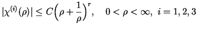
In this paper we are concerned with asymptotic behavior of the global solutions to the one-dimensinal Keller-Segel equations with a general sensitivity function satisfying $(\chi)$, and intend to construct an attractor set. In constructing the attractor we will use the theory of infinite dimensional dynamical systems for dissipative evolution equations which was developed in recent years by Temam [21] and by Eden, Foias, Nicolaenko and Temam [3,4]. In order to use their theory, the first step is to formulate (KS) as a semilinear evolution equation in a suitable Hilbert space. We set the underlying space $H$ as a product space of the pairs $\begin{pmatrix}u \\ \rho \end{pmatrix}$ with $u \in L^{2}(I)$ and $\rho \in H^{1}(I)$, and will show that the nonlinear semigroup constructed on $H$ satisfies some sufficient conditions which imply its crucial property called the squeezing property. As the result, will be shown existence of a compact set of finite fractal dimension which attracts solutions exponentially, such an attractor set is called the exponential attractor. 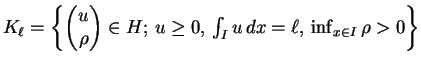However, we here notice that we can not expect any global compact attractor, for, since the norm $\Vert u(t) \Vert _{L^1} \equiv \Vert u_{0} \Vert _{L^1}$ is conserved for every $t \in [0, \infty)$, no compact set can attract every solution of (KS). Therefore, for each $\Vert u_{0} \Vert _{L^1} = \ell > 0$, we have to consider an underlying space like $K_{\ell} = \left\{ \begin{pmatrix}u \\ \rho \end{pmatrix} \in H; \, u \ge 0,\,\int_I u \, dx = \ell, \, \inf_{x \in I} \rho > 0 \right\}$ to reset.

In the case where the sensitivity function is linear, $\chi(\rho) = k \rho$, we know the existence of a global Lyapunov functional. Thanks to this we can obtain a result of another type, that is, for any initial data $\begin{pmatrix}u_{0} \\ \rho_{0} \end{pmatrix}\in K_{\ell}$, the $\omega$-limit set of the solution to (KS) contains at least one stationary solution. For other typical cases of $\chi(\rho)$, however, we do not know whether such a Lyapunov functional exists or not.

This paper is organized as follows. In Section 2, we recall the definition of the exponential attractor and the existence theorem of exponential attractors in the book [4]. We list also some results on the Sobolev spaces which we need in this paper. In Section 3, the local solutions of (KS) are constructed by applying the Galerkin method. In Section 4, we establish various a priori estimates of the local solutions. Section 5 is devoted to estimating the lower bound of $\rho$. By using these estimates, the existence of global solutions is verified. In Section 6, we prove the main theorem of the paper. Finally, Section 7 is devoted to considering the case where the sensitivity function is linear.

Notations. $I = (\alpha, \beta)$, $- \infty < \alpha < \beta < \infty$, denotes an open interval in $\mathbb{R}$. For $1 \le p \le \infty$, $L^{p}(I)$ is the $L^{p}$ space of measurable functions in $I$, its norm is denoted by $\Vert \cdot \Vert _{L^{p}}$. For $m = 0, 1,2, \cdots$, $H^{m}(I)$ is the real Sobolev space of exponent $m$, its norm is denoted by $\Vert \cdot \Vert _{H^{m}}$. More generally, $H^{s}(I)$ is the fractional Sobolev space which is the interpolation space between $H^{m}(I)$ and $H^{m + 1}(I)$ for $m < s < m + 1$, its norm is also denoted by $\Vert \cdot \Vert _{H^{s}}$. ${\cal C}({\overline{I}})$ is the space of all continuous functions on ${\overline {I}}$.

Let $X$ be a Banach space and let $J$ be an interval in $\mathbb{R}$. $L^2(J; X)$ and $H^{1}(J; X)$ are $X$-valued $L^2$ and $H^1$ space in $J$, respectively. ${\cal C}(J; X)$ and ${\cal C}^{m}(J; X)\ (m = 1,2,3,\cdots)$ denote the space of $X$-valued continuous functions and $m$-times continuously differentiable functions in $J$, respectively.

For simplicity, we will use a single notation $C$ to denote various constants determined by initial constants. $C$ is therefore determined in each occurrence by $I = (\alpha, \beta), a, b, c, d$ and $\chi$ in a certain specific way. In a case where $C$ depends also on some parameter, say $\varepsilon$, it will be denoted by $C_{\varepsilon}$.

Koichi Osaki, Atsushi Yagi